Reliable Effective Linear Learning

Project by Edward Chao (ID: 20474367), Prarthana Bhattacharyya (ID: 20714026) and Hari Govind V.K. (ID : 20743574).

Based on paper by Agarwal et al [1].

Problem Formulation
Proposed Optimization Algorithm
Dataset
Our Implemented Solution
Numerical Results
Visualizing the Results
Functions implemented
Analysis and Conclusions
References

Problem Formulation

Much of the work in machine learning focuses on linear learning problems of the form:

$min_{\textbf{w} \in R^d} {\sum_{i=1}^{n}{l(\textbf{w}^T\textbf{x}_i; y_i) + \lambda R(\textbf{w})}},$

where $\textbf{x}_i$ is the feature vector of the $i$ -th example, $y_i$ is the label, $\textbf{w}$ is the linear predictor, $l$ is a loss function and $R$ is a regularizer.

In order to optimize the objective function above when the number of examples $n$ is too large, pure online or pure batch learning algorithms have some drawbacks. For instance, although online learning algorithms optimize the objective to a rough precision quite fast, in just a handful of passes through the data, the inherent sequential nature of these algorithms makes them tricky to parallelize. Batch learning algorithms on the other hand are great at optimizing the objective to a high accuracy, once they are in a good neighbourhood of the optimal solution, but are quite slow in reaching this good neighbourhood. This paper thus proposes to use a hybrid online + batch algorithm with rapid convergence and small synchronization overhead for their parallel learning problem with large datasets.

Proposed Optimization Algorithm

The authors propose a hybrid online + batch algorithm as their main optimization technique for linear learning over large datasets. They make one online pass over the local data and each online pass occurs asynchronously. This helps them to get into a good neighbourhood of the optimal solution rather than recovering it to a high accuracy at the first stage. This solution for the weights $\bar {\textbf{w}}$ is used to initialize the batch learning algorithm with the expectation that the online stage gives it a good warmstart. This algorithm benefits from the fast initial reduction of the error provided by an online algorithm, and rapid convergence in a good neighbourhood guaranteed by quasi-Newton algorithms. In addition to the hybrid strategy, the authors also propose to evaluate repeated online learning with averaging using adaptive updates. They carry out several iterations, each of which has the following phases: (1) Pass through the entire local portion of the dataset and accumulate the result as a vector od size $d$ , i.e. the same size as the parameter vector (2) Do additional processing and updating of the parameter vector. The algorithm can be represented as follows:

Dataset

We use the CIFAR-10 dataset for demonstrating the implementation of proposed solution. The dataset can be downloaded from https://www.cs.toronto.edu/~kriz/cifar.html.

Our Implemented Solution

This section explains our implementation of the hybrid online + batch learning algorithm for optimizing the linear machine learning objective function.

% Clear all data
clc; clear all; close all;

%Load CIFAR-10 data
data1 = load('data_batch_1.mat');
data2 = load('data_batch_2.mat');
data3 = load('data_batch_3.mat');
data4 = load('data_batch_4.mat');
data5 = load('data_batch_5.mat');
data  = cat(1,data1.data,data2.data,data3.data,data4.data,data5.data);
labels = cat(1,data1.labels,data2.labels,data3.labels,data4.labels,data5.labels);
test_data = load('test_batch.mat');

%Setup parameters
data_length = 3072;  % value of dimension of input
num_classes = 10;    % CIFAR 10 classes
svm_buffer  = 1;     % loss threshold
step_size   = 0.001; % step size for gradient update
num_iters   = 10;    % number of iterations to run through
alpha       = 0.2;   % regularization parameters
random_W    = rand(num_classes, data_length); % initialize the weights

Pure online learning

% Timer for time taken by one online pass
tic
[online_W1, ll_online1] = onlineDescent(random_W,data_length,num_classes,svm_buffer,step_size*0.1,data,labels,alpha);
t_online = toc;
[online_W2, ll_online2] = onlineDescent(online_W1,data_length,num_classes,svm_buffer,step_size*0.1,data,labels,alpha);

Only batch learning

% Timer for time taken by the batch-update
tic
[batch_W, ll_batch, al_batch] = batchDescent(random_W,data_length,num_classes,svm_buffer,step_size,data,labels,num_iters,alpha,test_data.data,test_data.labels,0);
t_batch = toc;

Online and batch learning combined

[combined_W, ll_combined, al_combined] = batchDescent(online_W2,data_length,num_classes,svm_buffer,step_size,data,labels,num_iters,alpha,test_data.data,test_data.labels,0);

% Timer for time taken by hybrid method
tic
[combined_W_itr, ll_combined_itr, al_combined_itr] = batchDescent(online_W2,data_length,num_classes,svm_buffer,step_size,data,labels,num_iters,alpha,test_data.data,test_data.labels,1);
t_combined = toc;

Numerical Results

% Test  results
corr_perc_batch    = 100*eval_W(batch_W,    test_data.data, test_data.labels);
corr_perc_online   = 100*eval_W(online_W2,  test_data.data, test_data.labels);
corr_perc_combined = 100*eval_W(combined_W, test_data.data, test_data.labels);

% Test Accuracy
fprintf("Batch learning accuracy percentage: %f\n",corr_perc_batch);
fprintf("Online learning accuracy percentage: %f\n",corr_perc_online);
fprintf("Online + batch accuracy percentage: %f\n",corr_perc_combined);

% Time taken for learning
fprintf("\nTime for online pass in secs: %f\n",t_batch);
fprintf("Time for batch update in secs: %f\n",t_online);
fprintf("Time for online + batch learning in secs: %f\n",t_combined+t_online);

Batch learning accuracy percentage: 10.500000
Online learning accuracy percentage: 29.770000
Online + batch accuracy percentage: 31.320000

Time for online pass in secs: 0.409995
Time for batch update in secs: 30.059966
Time for online + batch learning in secs: 30.108000

Visualizing the Results

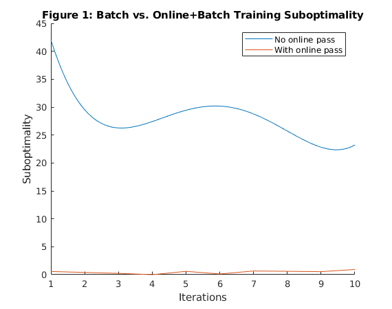
Plot the Suboptimality vs Iteration for only batch and online + batch method

figure
hold on
p = polyfit(1:num_iters, ll_batch-min(ll_combined), 4);
p_fun = polyval(p,1:0.1:num_iters);
plot (1:0.1:num_iters, p_fun)
title('Figure 1: Batch vs. Online+Batch Training Suboptimality')
plot(1:num_iters, ll_combined - min(ll_combined))
legend('No online pass', 'With online pass')
xlabel('Iterations')
ylabel('Suboptimality')
hold off

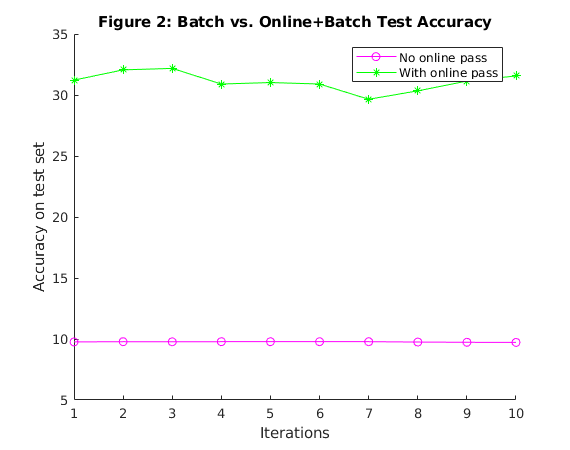
Plot the Test Accuracy vs Iteration for only batch and online + batch method

figure
hold on
plot(al_batch .* 100, 'm-o')
title('Figure 2: Batch vs. Online+Batch Test Accuracy')
plot(al_combined .* 100, 'g-*')
legend('No online pass', 'With online pass')
xlabel('Iterations')
ylabel('Accuracy on test set')

Functions implemented

Function to implement Online Learning

function [W, loss_log] = onlineDescent (initial_W,dl, nc, svmbuff, ss, data_train, label,alpha)
% Arrange the inputs
num_classes = nc;
svm_buffer  = svmbuff;
step_size   = ss;
data = data_train;
labels = label;
W = initial_W;
num_imgs = length(data);
loss_log = zeros(1,num_imgs);
  % For all local data
  for i = 1:num_imgs
    % Calculate score of image i
    img = im2double(data(i,:));
    score_i = W*img';
    % Get the label of image i
    y = double(labels(i));
    % Compute the objective function (hinge loss + regularization)
    tmp = score_i' - score_i(y+1) + svm_buffer;
    maxed = max(0,tmp);
    loss = sum(tmp)-svm_buffer + alpha*norm(W);
    loss_log(i) = loss;
    %Compute gradient
    bin_mask = find(maxed);
    bin_array = zeros(1,num_classes);
    bin_array(bin_mask) = 1;
    bin_array(y+1) = 0;
    % Parameter update
    gradient = bin_array' * img + alpha*2*W;
    W = W - step_size * gradient;
  end
end

Function to implement Batch Learning

function [W, loss_log, acc_log] = batchDescent (initial_W, dl, nc, svmbuff, ss, data_train, label, num_iters,alpha, test_data, test_label, flag)
% Arrange the inputs
data_length = dl;
num_classes = nc;
svm_buffer = svmbuff;
step_size = ss;
data = data_train;
labels = label;
num_iterations = num_iters;
W = initial_W;
batch_size = 16;
total_size = length(data);
num_imgs = batch_size;
loss_log = zeros(1,num_iterations);
acc_log = zeros(1,num_iterations);
 %For total number of epochs
  for j = 1:num_iterations
    total_loss = 0;
    total_gradient = zeros(num_classes, data_length);
    img_num = ceil(total_size.*rand(batch_size,1));
    %Calculate score of batch
    for k=1:length(img_num)
        img = im2double(data(img_num(k),:));
        score_i = W*img';
        %Get the label of image i
        y = double(labels(img_num(k)));
        % Compute objective
        tmp = score_i' - score_i(y+1) + svm_buffer;
        maxed = max(0,tmp);
        total_loss = total_loss + sum(maxed)-svm_buffer + alpha*norm(W);
        %Accumulate gradient
        bin_mask = find(maxed);
        bin_array = zeros(1,num_classes);
        bin_array(bin_mask) = 1;
        bin_array(y+1) = 0;
        total_gradient = total_gradient + bin_array' * img + alpha*2*W;
    end
    % Parameter update
    average_loss = total_loss / num_imgs;
    average_gradient = total_gradient / num_imgs;
    W = W - step_size * average_gradient;
    % Evaluate the accuracy of test data
    loss_log(j) = average_loss;
    acc_log(j) = eval_W(W, test_data, test_label);
    if flag == 1 && acc_log(j) > 0.3
        break;
    end
  end
end

Function to evaluate the accuracy of test data

function eval = eval_W(W, data, labels)
% Test results
data = im2double(data);
test_scores = W * data';
%Find predicted classes
[M, I] = max(test_scores,[],1);
%Compare predicted classes to ground truth
evaluation = I-(double(labels')+1);
idx = evaluation==0;
num_corr = sum(idx);
%Calculate accuracy
eval = num_corr / length(labels');
end

Analysis and Conclusions

We implemented the online + batch optimization approach proposed by [1] for reliable linear learning on large datasets. We now investigate the speed of convergence of three different learning strategies: batch, online and hybrid. We are also interested in how these algorithms maximize the test accuracy.

Figure 1 compares how fast the two learning strategies - batch with and without an initial online pass - optimize the training objective. It plots the optimality gap, defined as the difference between the current objective function and the optimal one, as a function of the number of iterations. We can see that the initial online pass helps the batch reduce the optimal value within very few iterations. Figure 2 shows the test accuracy with only batch updates and batch + online pass. The hybrid approach seems to be the most effective in terms of minimizing the test error. We also note that the hybrid method takes only a few seconds more than the purely online method but gives a higher test accuracy. We also check that this is the state of the art accuracy for linear learning on CIFAR 10.

We thus conclude that we have replicated the results shown in the paper [1]. We found that online learning is fast but since it is hard to parallelize, the parameter estimate obtained from an online pass can be used to warmstart the batch learning process. The batch learning technique converges to a very accurate estimate once it is in a good neighbourhood of the solution as shown by our experiment. Thus the hybrid online + batch method is the most effective approach and gives a more accurate solution while using up very little time overhead, allowing it to be parallelized and used for large datasets.

References

[1] Alekh Agarwal, Olivier Chapelle, Miroslav Dudik, and John Langford. A Reliable Effective Terascale Linear Learning System. Journal of Machine Learning Research, 2012. www.jmlr.org/papers/volume15/agarwal14a/agarwal14a.pdf

[2] Boyd, Stephen, and Lieven Vandenberghe. Convex Optimization. Cambridge University Press, 2004.