Hand-Eye Calibration using Convex Optimization
Barry Gilhuly (88075397), Abhinav Dahiya (20753240)
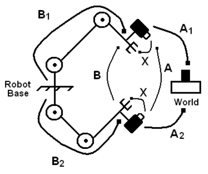
In robotics, cameras are frequently mounted directly to the end-effector of the robot. However, due to the complexities of the joints, differences in cameras and other variations, it is impossible to directly measure the translation from the camera to the end-effector. As an alternative to an imprecise measurement, Shiu and Shaheen [2] discovered a method to iteratively calculate the translation using sequential camera/robot poses.
The paper we selected [1] discusses an alternate method which uses the Infinity norm and convex optimization to find a better result, in less computational time.
Contents
- Problem Formulation
- Proposed solution
- Data sources
- Solution
- Generating Data
- Solving with CVX
- Calculating the Error
- The complete solution
- Visualization of results
- Analysis and conclusions
- Source Reference
- References
- Supporting Functions
- [A, B, C ,d] = buildMinimizationData( Xact, sigma, samples )
- [delta,x] = runCVX( C, d )
Problem Formulation
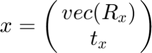
The relationship between the camera's frame of reference and that of the robot's end effector can be expressed as an equation of transformation matrices:

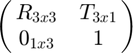
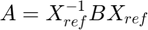
where A is the transformation from the Camera to the world frame, B is the transformation from the robot base to the end effector, and X is the unknown transformation from the Camera to the end effector. Each of the matrices is a combination of rotation and translation of the form:
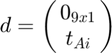
The hand-eye calibration equation can then be split into two equations -- one of rotation only, and one of rotation and translation:


Using the Infinity Norm, the calibration problem posed by these two equations becomes one of convex optimization:
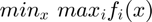
where  is an error function that takes
one of two forms: orthonormal or quaternian. While the author
implemented both forms in his paper, we've elected to simulate
orthonormal only.
is an error function that takes
one of two forms: orthonormal or quaternian. While the author
implemented both forms in his paper, we've elected to simulate
orthonormal only.
Proposed solution
In the orthonormal solution, the infinity norm min/max problem can be expressed in standard form as an SOCP:


where C and d are a re-arrangement of the calibration equations.
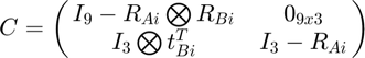
 represents the Kronecher
multiplication function. Using simulated data, this SOCP can be
solved using CVX and MATLAB.
represents the Kronecher
multiplication function. Using simulated data, this SOCP can be
solved using CVX and MATLAB.
Data sources
The authors of the paper do not provide access to the data set they used to simulate motion, nor do they clearly explain how they generated their data. However, referring to [2] gave us some ideas.
Assuming the Hand-eye setup from [2], we constructed a set of n robot motions, at several noise levels, using the following method:
- From the original paper [2], start with the stated value for Xact, the actual transformation from the camera to the end-effector.
- Select a random angle to use as the base angle for this iteration.
- Using the base angle, add Gaussian noise, and construct the A transformation matrix.
- Construct an alternate A, A_alt, using a different value for noise. Using A_alt and the known relationship between A, Xact, and B, calculate a value for B using the equation:
- Using our values for A and B, construct C and d.
% Our value for X_act
%
Xact = [  1.0  0.000000  0.000000  10;
          0.0  0.980067 -0.198669  50;
          0.0  0.198669  0.980067 100;
          0    0         0          1];
Ract = Xact(1:3,1:3);
Tact = Xact(1:3,4);
Solution
Generating Data
We're using CVX to solve the minimization problem. First we build some sample data.
[ A, B, C, d ] = buildMinimizationData( Xact, 0.01, 10 );
Solving with CVX
Next we minimize delta, subject to our constraints, with variables x, and delta.
cvx_begin
    variables x(12,1) delta(1)
    minimize (delta)
    subject to
        for j = 1:size(C,1)
            norm( C{j}*x - d{j} ) <= delta;
        end
cvx_end
A representitive sample of CVX output:
    Calling SDPT3 4.0: 132 variables, 23 equality constraints
       For improved efficiency, SDPT3 is solving the dual problem.
    ------------------------------------------------------------

     num. of constraints = 23
     dim. of socp   var  = 122,   num. of socp blk  = 10
     dim. of linear var  = 10
    *******************************************************************
       SDPT3: Infeasible path-following algorithms
    *******************************************************************
     version  predcorr  gam  expon  scale_data
        NT      1      0.000   1        0
    it pstep dstep pinfeas dinfeas  gap      prim-obj      dual-obj    cputime
    -------------------------------------------------------------------
     0|0.000|0.000|2.0e+01|4.1e+00|1.4e+04| 0.000000e+00  0.000000e+00| 0:0:00| chol  1  1
     1|1.000|1.000|1.8e-03|1.5e-03|3.7e+02|-2.389950e-03 -3.721369e+02| 0:0:00| chol  1  1
     2|1.000|0.986|6.5e-08|5.2e-04|5.3e+00|-3.243462e-03 -5.209168e+00| 0:0:00| chol  1  1
     3|1.000|0.782|2.3e-08|1.2e-04|1.2e+00|-1.248165e-01 -1.271622e+00| 0:0:00| chol  1  1
     4|0.694|0.639|2.4e-07|4.6e-05|4.4e-01|-5.637747e-01 -9.969178e-01| 0:0:00| chol  1  1
     5|0.840|0.892|4.6e-08|5.1e-06|6.6e-02|-7.180699e-01 -7.838007e-01| 0:0:00| chol  1  1
     6|0.899|0.851|7.7e-08|7.8e-07|9.2e-03|-7.419227e-01 -7.510263e-01| 0:0:00| chol  1  1
     7|0.895|0.874|5.3e-08|1.1e-07|1.3e-03|-7.452468e-01 -7.465466e-01| 0:0:00| chol  1  1
     8|0.890|0.863|5.6e-08|2.6e-08|2.0e-04|-7.457212e-01 -7.459138e-01| 0:0:00| chol  1  1
     9|0.948|0.945|3.1e-08|1.1e-08|1.4e-05|-7.457875e-01 -7.458000e-01| 0:0:00| chol  1  1
    10|0.967|0.945|1.1e-09|1.2e-09|9.3e-07|-7.457921e-01 -7.457928e-01| 0:0:00| chol  1  1
    11|0.981|0.947|2.5e-09|1.0e-10|6.1e-08|-7.457923e-01 -7.457924e-01| 0:0:00| chol  1  2
    12|0.511|0.894|1.3e-09|2.1e-11|1.5e-08|-7.457923e-01 -7.457924e-01| 0:0:00|
      stop: max(relative gap, infeasibilities) < 1.49e-08
    -------------------------------------------------------------------
     number of iterations   = 12
     primal objective value = -7.45792312e-01
     dual   objective value = -7.45792372e-01
     gap := trace(XZ)       = 1.55e-08
     relative gap           = 6.21e-09
     actual relative gap    = 2.42e-08
     rel. primal infeas (scaled problem)   = 1.33e-09
     rel. dual     "        "       "      = 2.12e-11
     rel. primal infeas (unscaled problem) = 0.00e+00
     rel. dual     "        "       "      = 0.00e+00
     norm(X), norm(y), norm(Z) = 9.5e-01, 1.1e+02, 3.2e+00
     norm(A), norm(b), norm(C) = 8.7e+02, 2.0e+00, 3.1e+02
     Total CPU time (secs)  = 0.15
     CPU time per iteration = 0.01
     termination code       =  0
     DIMACS: 1.3e-09  0.0e+00  6.6e-11  0.0e+00  2.4e-08  6.2e-09
    -------------------------------------------------------------------

    ------------------------------------------------------------
    Status: Solved
    Optimal value (cvx_optval): +0.745792
Calculating the Error
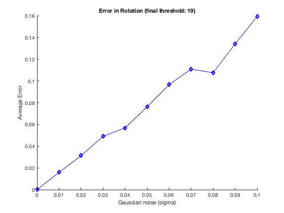
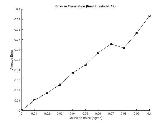
For each iteration, the errors in rotation and translation are calculated separately. The error in rotation is calculated:
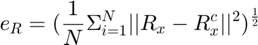
And the translation error is:
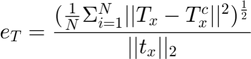
The comparison of these errors vs. input noise is shown in the two graphs that follow.
The complete solution
We've written a function to encapsulate the simulation and return the measured error results in a pair of arrays. For our simulation, at each level of noise, we'll generate 10 samples for each iteration, and run 100 iterations.
samples = 10;
iterations = 100;
epsilon = 1;          % Our initial (minimum) threshold
sigmaStep = 0.01;    % The step value for sigma of our gausian noise function ~N(0,sigma^2)
[eR_S, et_S, epsilon] = runSimulation( samples, iterations, epsilon, sigmaStep );
Visualization of results
Our results are similar to those of the researcher, and meet our expectations. Not surprisingly, the measured error increases as more noise is introduced into the system. The resulting minimum threshold required to run the test is displayed in the title of each graph.
figure(1); clf; hold on;
plot([0:sigmaStep:0.1], eR_S, 'bd-')
xlabel( 'Gaussian noise (sigma)' );
ylabel( 'Average Error' );
str = sprintf( 'Error in Rotation (final threshold: %d)', epsilon );
title( str );
figure(2); clf; hold on;
plot([0:sigmaStep:0.1], et_S, 'ks-')
xlabel( 'Gaussian noise (sigma)' );
ylabel( 'Average Error' );
str = sprintf( 'Error in Translation (final threshold: %d)', epsilon );
title( str );
Analysis and conclusions
We were successful in recreating the results from our paper.
However, the information presented was unclear, requiring
us to reference the original paper where this problem was first
raised and solved. We investigated implementing the second
formulation using quaternions, as the author claimed it was just as
fast, but more accurate. In order to implement the quaternion
solution as a convex optimization, the author needed to enforce the
constraint  . He did this by
introducing a new constraint:
. He did this by
introducing a new constraint:

but other than a hand wave of the unit quaternion constraint and "some apriority [sic] knowledge", failed to define the either the matrix D or f. Without this information, we were unable to procede with the second formulation.
The first formulation of the algorithm was straightforward to implement and behaved as expected. Our results are a close parallel to what the author produced.
After observing how the algorithm behaves, we aren't convinced that the author's method is entirely correct. Specifically, the introduction of a threshold to accomodate incorrect/unsuitable transformations [3] seems somewhat suspect. Here is the algorithm as written in the paper:
Given the motion data set C = { C1, C2, ... Cn },
d = { d1, d2, ..., dn } and the threshold e
Repeat
Solve the SOCP For each motion in C,d:
If 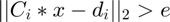 Remove
  from the set
Until delta <= e
from the set
Until delta <= e
Removing any motions that generate a value greater than the minimum is a quick way to ensure that all of your data fits within your expectations.
The author doesn't suggest a value for the threshold, although some testing with noise suggests the reason for that: as the noise level is increased, the minimum value of delta increases. If the threshold is too tight, all of the samples are eliminated and no results are generated.
Since there are no recommendations in the paper regarding the value of the threshold, we've implemented one that slowly increases as required. On any iteration, if the threshold causes all of the samples to be eliminated, we increase the threshold slightly and recreate a new set of measurements.
On the chart, the average error increases every time the threshold is relaxed. At the very least, the fact that the minimum value of delta increases with as the noise increases suggests that this algorithm is very sensitive to noise.
Some further reflection on motion data selection [3] may shed a little light on what the author is attempting to do. It seems that with motion analysis, not all motions are suitable for generating an accurate estimate of the hand-eye transformation. The author of [1] also comments on this, suggesting that without good starting data, the Euclidean iterative solutions are likely to end up in a global minimum.
Source Reference
A list of (linked) custom source files/functions necessary for your implementation of the algorithm.
function [eR_S, et_S, epsilon] = runSimulation( samples, iterations, epsilon, sigmaStep )
    Xact = [1.0       0.000000  0.000000  10;
            0.00      0.980067 -0.198669  50;
            0.000000  0.198669  0.980067 100;
            0         0         0          1];
    Ract = Xact(1:3,1:3);
    Tact = Xact(1:3,4);

    eR_S = [];
    et_S = [];

    % Step through the noise levels, running the an iteration for each
    % value of sigma.
    for sig = 0:sigmaStep:0.1
        eR = 0;
        et = 0;

        for itr = 1:iterations

            % Calculate the data for this iteration based on Xact, the
            % noise level, sigma, and the number of samples requested
            [ A, B, C, d ] = buildMinimizationData( Xact, sig, samples );

            % Main algorithm from paper
            while true
                % run the minimization
                [delta, x] = runCVX( C, d );

                % if the results were acceptable, exit
                if ~epsilon || delta <= epsilon
                    break;
                end

                % check for any outliers and remove them
                for s = length(C):-1:1
                    if norm( C{s} * x - d{s} ) > epsilon
                        C(s) = [];
                        d(s) = [];
                        A(s) = [];
                        B(s) = [];
                    end
                end

                % If the threshold, epsilon, is too low, all of the data
                % will be eliminated due to noise.  If this happens, the
                % value for the threshold must be increased and the trial
                % run again.
                if length(C) < 0.5*samples
                    epsilon = epsilon + 1;
                    fprintf( "Increasing threshold to %d\n", epsilon );
                    [ A, B, C, d ] = buildMinimizationData( Xact, sig, samples );
                end
            end

            Rx = reshape(x(1:9), [3,3])';
            Tx = x(10:12);

            % calculate the error residue and add it to the total
            eR = eR + norm(Rx - Ract)^2;
            et = et + norm(Tx - Tact)^2;
        end

        % calculate the error for the current noise constraint
        eR = sqrt(eR/iterations);
        et = sqrt(et/iterations) / norm( Tact );

        eR_S = [eR_S; eR];
        et_S = [et_S; et];
    end
end
References
[1] - Zhao, Zijian. "Hand-eye calibration using convex optimization." Robotics and Automation (ICRA), 2011 IEEE International Conference on. IEEE, 2011.
[2] - Shiu, Yiu Cheung, and Shaheen Ahmad. "Calibration of wrist-mounted robotic sensors by solving homogeneous transform equations of the form AX= XB." IEEE Transactions on robotics and automation 5.1 (1989): 16-29.
[3] - Schmidt, Jochen, and Heinrich Niemann. "Data selection for hand-eye calibration: a vector quantization approach." The International Journal of Robotics Research 27.9 (2008): 1027-1053.
[4] - Shah, Mili, Roger D. Eastman, and Tsai Hong. "An overview of robot-sensor calibration methods for evaluation of perception systems." Proceedings of the Workshop on Performance Metrics for Intelligent Systems. ACM, 2012.
[5] - Grant, Michael, Stephen Boyd, and Yinyu Ye. "CVX: Matlab software for disciplined convex programming." (2008).
Supporting Functions
These two function implement the main parts of our simulation: the generation of data samples, and the actual CVX minimization sequence.
[A, B, C ,d] = buildMinimizationData( Xact, sigma, samples )
Calculate the Camera position, Arm position, and required matrices for minimization, including a given Gaussian disturbance.
function [A, B, C ,d] = buildMinimizationData( Xact, sigma, samples )
    A = cell(samples,1);
    B = cell(samples,1);
    C = cell(samples,1);
    d = cell(samples,1);

    for i = 1:samples

        % Calculate an initial translation for the robot arm
        theta = pi*rand();

        % Add noise to theta and calculate the A matrix
        thetaA = theta + normrnd(0,sigma);
        ct = cos(thetaA);
        st = sin(thetaA);

        % The paper comments that for the solution to be unique,
        % subsequent rotations should be in an alternate plane
        if mod(i,2)==0
            Ra = [ct -st 0;
                st ct 0;
                0 0 1];
        else
            Ra = [ct 0 st;
                0 1 0;
                -st 0 ct];
        end

        % Choose a random displacement
        tx = 1 * (100 - 200*rand());
        ty = 1 * (100 - 200*rand());
        tz = 1 * (100 - 200*rand());
        Ta = [tx; ty; tz];

        % Construct A
        A{i} = [Ra Ta; [0 0 0 1]];

        % In order to calculate B, a separate A with a different noise variation
        % must be constructed.  Vary the rotation on sequential samples.
        thetaB = theta + normrnd(0,sigma);
        ct = cos(thetaB);
        st = sin(thetaB);
        if mod(i,2)==0
            RBa = [ct -st 0;
                st ct 0;
                0 0 1];
        else
            RBa = [ct 0 st;
                0 1 0;
                -st 0 ct];
        end

        % Construct A using the new rotation component and the same
        % translation
        Ab = [RBa Ta; [0, 0, 0, 1]];

        % Calculate B using the relationship between A, B, and Xact
        B{i} = Xact\Ab*Xact;
        Rb = B{i}(1:3,1:3);
        Tb = B{i}(1:3,4);

        % Calculate the C and d matrices
        C{i} = [eye(9)-kron(Ra,Rb) zeros(9,3); kron(eye(3),Tb') eye(3)-Ra];
        d{i} = [zeros(9,1); Ta];
    end

end
[delta,x] = runCVX( C, d )
Run a single minimization and return the result
function [delta, x] = runCVX( C, d )
    cvx_begin quiet
        variables x(12,1) delta(1)
        minimize (delta)
        subject to
            for j = 1:size(C,1)
                norm( C{j}*x - d{j} ) <= delta;
            end
    cvx_end
end