ECE602 Project: Optimal Energy Allocation for Wireless Communication With Energy Harvesting Constraints
Submitted by: Jiayin Chen (20699444) and Mushu Li (20450182)
Contents
- 1. System Model
- 2. Problem Formulation
- 3-1. Problem Solution: Causal Side Information and Full Side Information with Finite Battery Size
- 3-2. Problem Solution: Full Side Information with Infinite Battery Size
- 4. Data Source
- 5. Visualization of Results
- 6. Result Analysis & Conclusion
- Appendix: Function for Causal SI with AWGN Channel
- Appendix: Function for Causal SI with Fading Channel
- Appendix: Function for Full SI with AWGN or Fading Channel
- Appendix: Functions for Throughput Comparision Between Water-filling and Power-halving Schemes
- Reference
1. System Model
The work [1] introduces the power allocation in the wireless communication transmitter with energy harvest device. The main objective is maximizing the mutual information over time slot with the energy harvest constraint, which the harvested energy in future time slots can not be used in the past time slot, i.e., causality. Assume that one packet transmission is performed in each time slot, which allows  symbols to be transmitted. The slot index is represented by the slot index
  . In slot
  , a message
  is sent. Consider slot
  . The battery has available
  amount of stored energy per symbol. For transmission, the message
  is first encoded as data symbols
 ![$$X^{n}_{k} = [ X_{1k} , ... , X_{nk} ]$](main_published_eq83259.png) of length , where we normalize
of length , where we normalize  . Then, the transmitter transmits packet in slot as
  , where
  is the energy per symbol used by the power amplifier.
In this project, there are two scenarios are discussed: Causal Side Information (Causal SI) available and Full Side Information (Full SI) available. With Casual SI, the power allocation is analyzed under the constraint that only current channel state and battery level available. To allocate the power with causal information, the dynamic of the system need to be predicted with Markov model, which we will discuss as follows. In Full SI scenario, the channel state and the energy harvest details are fully available for all time slots. The only constraint in the full SI problem is the energy harvest constraint. The power allocation with full SI can be modeled by optimization equation straightforward, which referred to the Section 3.
1. Mutual Information
The channel is quasistatic for every slot with SNR  . The maximum reliable transmission rate in slot is then given by the mutual information
  in bits per symbol. In general, given
  ,
,  is concave and non-descreasing in
  as following equation:
2. Battery Dynamics
The battery energy from slot 1 to slot is denoted by ![$$\mathit{B}^{k} = [\mathit{B}_{1} , ... , \mathit{B}_{k} ]$](main_published_eq88623.png) . The energy harvester collects an average energy of
. The energy harvester collects an average energy of  per symbol, which is then stored in the battery. At time instant
  , the stored energy increases and decreases linearly under the constraint that maximum stored energy
  in the battery cannot exceeded, which is shown as following equation:

We assume the initial stored energy  is known, where
  .
.
3. Channel and Harvest Dynamics
With casual side information available scenario, to model the unpredictable nature of energy harvesting and the wireless channel over time, we model  and
and  jointly as a random process described by their joint distribution. The SNR
  and the harvested energy
  are assumed to be constant in each slot and follow a first-order stationary Markov model over time . Given
  and
and  , the joint pdf of and is:


In this report, we assume that the joint distribution is known, which may be obtained via long-term measurements in practice.
4. Overall Dynamics:
Let us denote the state  , or simply
  if the index is arbitrary. Let the accumulated states be
  . Furthermore, we assume the initial state
  to be always known by the transmitter, which may be obtained causally prior to any transmission. given
  , the states thus follow a first-order Markov model:

2. Problem Formulation
1. Causal Side Information
Consider the case of causal SI, in which the transmitter has knowledge of  before packet is transmitted, where . At slot , the transmitter only knows the present channel SNR , past harvested energy
  , and present energy stored in the battery
  .
.
The causal SI is used to decide the amount of energy  for transmitting packet . To maximize the throughput, i.e.,the expected mutual information summed over a finite horizon of
  time slots, a deterministic power allocation policy is chosen by following equation:
 .
.
A policy is feasible if the energy harvesting constraint  is satisfied for all possible
  and all . We denote the space of all feasible policies as
  . Mathematically, given
  , the maximum throughput is
where, ![$$\mathcal{T} (\pi) = \sum_{k=1}^{K} \mathbf{E} [\mathit{I}(\gamma_k,\mathit{T}_{k}(s_k)) \mid s_1, \pi].$](main_published_eq42830.png)
The  summation term represents the throughput of packet at time slot (after expectation); its expectation is performed over all (relevant) random variables given initial state and policy
  . In general the optimization of power allocation,
  cannot be performed independently due to the energy harvesting constraints. If
  , we can first optimize
  with the knowledge of all possible power allocation in the first time slot,
  , (and hence all possible
  ), then optimize with the optimal (as a function of ).
2. Full Side Information
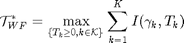
Without the constraint of the battery capacity, the throughput maximization can be formulated as the following objective function:
From the time slots 1 to  , the power allocation
  can only utilize the energy from current battery capacity, which is denoted as the summation of initial battery capacity
  and the harvested energy in past time slots
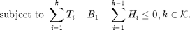
  . The energy harvest constraint represents that the optimal power allocation always keeps the battery level nonnegative for the next time slot. Therefore, there are
  number of constraints in the throughput optimization the problem from time slot 1 to
  .
.
3-1. Problem Solution: Causal Side Information and Full Side Information with Finite Battery Size
Given initial state  , the maximum throughput
  is given by
  , which can be computed recursively based on Bellman's equations, starting from
  ,
,  , and so on until :

and

For  , where
 ![$$\bar{\mathit{J}}_{k+1} (\gamma,\mathit{H},x) = \mathbf{E}_{\tilde{\mathit{H}},\tilde{\gamma}} [\mathit{J}_{k+1} (\tilde{\gamma},\tilde{\mathit{H}},min\{\mathit{B}_{max}, x + \tilde{\mathit{H}}) \mid \gamma,\mathit{H}]$](main_published_eq03721.png) .
.
The term  denotes the harvested energy in the present slot given the harvested energy
  in the past slot, and
  denotes the SNR in the next slot given the SNR in the present slot.
An optimal policy is denoted as  ,
,  is the optimal
  that solves the problem above.
If we assume a Rayleigh fading channel with expected SNR given by  , the expected mutual information evaluates as
![$$\bar{\mathit{I}} (\mathit{T}) = \mathbf{E}_{\gamma} [ \mathit{I} (\gamma,\mathit{T})] = exp (\frac{1}{\bar{\gamma}\mathit{T}}) E_1(\frac{1}{\bar{\gamma}\mathit{T}}) / ln(2),$](main_published_eq42788.png)
where the exponential integral is defined as  .
.
If we assume an AWGN channel where the channel is time-invariant with  for all , then the expected mutual information is simplied as:
 .
.
- Algorithm Implementation:
- First obtain
 via the closed-form results for AWGN or Rayleigh fading channel, we drop the and arguments due to the i.i.d. assumption.
 - Then we obtain
 , by an iterative bisection method. The throughput are averaged over
  independent realizations of and to give
  . This procedure is performed for different
  , discretized in step size of 0.01, and stored to be used for the next recursion.
 - The iteration is repeated for
 .
.
3-2. Problem Solution: Full Side Information with Infinite Battery Size
To solve the objective function with the energy harvest constraint efficiently, the conventional water-filling algorithm can be developed to adopt the energy harvest constraint. In the conventional water-filling algorithm, the throughput is maximized with a fixed power constraint over all time slots. Therefore, firstly, we introduce the conventional water-filling algorithm without the energy harvest constraint. Furthermore, we will introduce the staircase water-filling algorithm proposed in [1], which transforms the conventional water-filling algorithm to solve the energy harvest problem.
1. Conventional Water-filling Algorithm
The water-filling algorithm is a well-known algorithm in the information theory field, which maximized the channel capacity with an overall power constraint. The conventional problem can be summarized as follows:
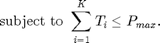
In the conventional water-filling problem, there is only one constraint, which the overall allocated power cannot over the power budget  . The closed form solution for the conventional water-filling problem can be derived by Karush-Kuhn-Tucker (KKT) conditions, where
![$$ {T}_{WF,k}^* = \Big[ \nu - \frac{1}{\gamma_k} \Big]^+$](main_published_eq90898.png) . The optimization parameter
. The optimization parameter  can be visualized as the water level, which is introduced by the Lagrangian multiplier. is a constant over the time slots. The allocated power can be visualized as the water in the water tank, and the inverse of SNR can be visualized as the stairs at the bottom of the water tank. The summation between optimal power allocation and the inverse of SNR is a constant number over the time slots. More power will be allocated to the time slots with higher SNR, and less power will be allocated to the time slots with lower SNR. If the optimal water level can be derived, the power allocation over time slots can be found effectively. The water-filling algorithm is proposed to search the water level with satisfying the overall power budget. However, the objective function of conventional water-filling has less constraint compared to the main objective function for energy harvest problem, which cannot ensure the optimal power allocation with causality manner.
2. Staircase Water-filling Algorithm
Due to the causality of the energy harvest problem, the conventional water-filling algorithm cannot handle the energy harvest constraint. Therefore, the work [1] proposed a staircase water-filling algorithm.
The objective function in Section 3 can be transformed to the dual composition problem as follows:
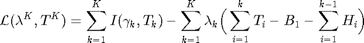 $,
$,
where the optimal power allocation  , and the Lagrangian mutiplier
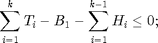
  . The KKT conditions for the primal and dual optimal are summerized as follows:
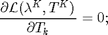


Then we can get the optimal power allocation result:
![$$ {T}_{k}^* = \Big[ \nu_k - \frac{1}{\gamma_k}
\Big]^+,$$ where $$\nu_k = (\textrm{ln}2 \sum_{i=k}^K \lambda_i)^{-1}.$$](main_published_eq30709.png)
Distinguished with the conventional water-filling solution, the water level  is a time-dependent value. The water level in time slot is adjusted only if the Lagrangian multiplier
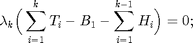
  , and we denoted the slot is transition slot (TS). From KKT condition and complementary slackness condition, we can get:
and
i.e., the battery is emptying at TS. Furthermore, the water level integral the past  , and is non-negative value. Therefore, the water level is a non-decreased by the time, and the water level will maintain as a constant among time slots excepting TSs. At TS, the water level will jump to a higher level. Overall, the water level is increasing as the staircase like. From the non-decreased water level, we can see that if the SNR for the channel is non-decreased by the time, the power allocation is non-decreasing over slots.
As mentioned above, the convention water-filling problem has an efficient algorithm to allocate the power by searching the water level. We observe that, in the staircase water-filling problem, the water-level is piecewise constant, and only jumped at TSs, and the battery is emptying at TS. Therefore, in the interval of two TS, the water level is constant, and the overall power budget is the harvested power inside the interval. Therefore, we can solve the staircase water-filling problem by combining multiple conventional water-filling problems. Denote  is the i-th TS, and
  is the set for the time slots between TS
  and . The optimal power allocation can be transformed to the conventional water-filling problem as follows:

where  is the harvested energy in the x-th TS interval, and the power constraint in the
  interval cannot violate the casualty constraint in the energy harvest problem at each time slot. Then, if the optimal TS is available, the power allocation can be achieved by running the water-filling algorithm with polynomial time.
The feasible search method is utilized in [1] for searching the optimal TS. Firstly, the forward-search is performed to find all possible TSs, from  to
to  . In each TS searching iteration, a backward-search is executed to find the maximum time slot can performing conventional water-filling algorithm without violating the energy harvest constraint.
4. Data Source
The data source is obtained from the original work [1]. AWGN and Rayleigh channel models are analyzed, and the SNR $ and harvested energy  are considered as i.i.d. over time slots. The harvested energy by the time slots is selected from {0,0.5,1} with equal probability, and the battery capacity is considered as infinity.
5. Visualization of Results
Firstly, the results from causal SI and full SI are compared under AWGN and Rayleigh fading channel respectively. The figures depict the comparison between full SI and causal SI with the mean SNR from 0 to 20. The simulation is examined with various time slot number: K = 1, 2 and 4. The corresponding code for functions are attached in the appendix. Same as the paper, the result is averaging from the results in 10^4 Monte Carlo runs.
clc
clear all
MC_run_1 = 1e4; %Monte Carlo Run for Fig 4,5
MC_run_2 = 2e4; %Monte Carlo Run for Fig 7
I_res_awgn(1,:) = FSI_SNR(1,MC_run_1,1);
I_res_awgn(2,:) = FSI_SNR(2,MC_run_1,1);
I_res_awgn(3,:) = FSI_SNR(4,MC_run_1,1);
I_res_ray(1,:) = FSI_SNR(1,MC_run_1,2);
I_res_ray(2,:) = FSI_SNR(2,MC_run_1,2);
I_res_ray(3,:) = FSI_SNR(4,MC_run_1,2);
fprintf('Finished: Fig 4 AWGN and Fig 5 Fading channel with full SI')

% Fig 4 AWGN and Fig 5 Fading channel with Causal SI
% Bellman Equation
Thrpt_AWGN_CSI(1,:)=CSI_AWGN_SNR(1,MC_run_1);
Thrpt_AWGN_CSI(2,:)=CSI_AWGN_SNR(2,MC_run_1);
Thrpt_AWGN_CSI(3,:)=CSI_AWGN_SNR(4,MC_run_1);
Thrpt_Ray_CSI(1,:)=CSI_Ray_SNR(1,MC_run_1);
Thrpt_Ray_CSI(2,:)=CSI_Ray_SNR(2,MC_run_1);
Thrpt_Ray_CSI(3,:)=CSI_Ray_SNR(4,MC_run_1);
fprintf('Finished: Fig 4 AWGN and Fig 5 Fading channel with Causal SI')


% GRAPH: Fig 4 and Fig 5

figure(1)
hold on
grid on
plot(0:5:20,I_res_awgn(1,:),'-or','LineWidth',2)
plot(0:5:20,I_res_awgn(2,:),'-og','LineWidth',2)
plot(0:5:20,I_res_awgn(3,:),'-ob','LineWidth',2)
plot(0:5:20,Thrpt_AWGN_CSI(1,:),'-xr','LineWidth',2)
plot(0:5:20,Thrpt_AWGN_CSI(2,:),'-xg','LineWidth',2)
plot(0:5:20,Thrpt_AWGN_CSI(3,:),'-xb','LineWidth',2)
legend({'Full SI, K=1','Full SI, K=2','Full SI, K=4','Causal SI, K=1','Causal SI, K=2','Causal SI, K=4'} ,'Location','southeast')
xlabel('SNR(dB)')
ylabel('Throughput pre slot')
title('AWGN channel (Fig. 4)')

figure(2)
hold on
grid on
plot(0:5:20,I_res_ray(1,:),'-or','LineWidth',2)
plot(0:5:20,I_res_ray(2,:),'-og','LineWidth',2)
plot(0:5:20,I_res_ray(3,:),'-ob','LineWidth',2)
plot(0:5:20,Thrpt_Ray_CSI(1,:),'-xr','LineWidth',2)
plot(0:5:20,Thrpt_Ray_CSI(2,:),'-xg','LineWidth',2)
plot(0:5:20,Thrpt_Ray_CSI(3,:),'-xb','LineWidth',2)
legend({'Full SI, K=1','Full SI, K=2','Full SI, K=4','Causal SI, K=1','Causal SI, K=2','Causal SI, K=4'},'Location','southeast')
xlabel('SNR(dB)')
ylabel('Throughput pre slot')
title('Fading channel (Fig. 5)')
Elapsed time is 5.240421 seconds.
Elapsed time is 13.579237 seconds.
Elapsed time is 33.005100 seconds.
Elapsed time is 6.336301 seconds.
Elapsed time is 16.267225 seconds.
Elapsed time is 37.794627 seconds.
Finished: Fig 4 AWGN and Fig 5 Fading channel with full SIElapsed time is 0.242561 seconds.
Elapsed time is 16.765536 seconds.
Elapsed time is 20.792958 seconds.
Elapsed time is 24.730536 seconds.
Elapsed time is 1176.220712 seconds.
Elapsed time is 40432.455667 seconds.
Finished: Fig 4 AWGN and Fig 5 Fading channel with Causal SI


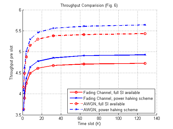
Furthermore, the optimal throughput under full SI scenario is compared with the power halving scheme. The power having scheme allocates the power in each time slot from the half of the current battery capacity, which is independent with the SNR of the channel. However, it is also an efficient power allocation scheme since it defers the battery energy to the further power allocation, which is similar with the staircase water-filling with non-decreased water level for further power allocation. Different with the Bellman equation method for causal SI, the staircase water-filling method for full SI has much lower computational complexity. Therefore, in this figure, the number of time slots  is increased from 0 to
  , and the mean SNR is fixed as 20 dB. Same as the paper, we run
  Monte Carlo simulations and plot the average of results.
I_ph_Rayleigh = TS_ph(MC_run_2,2);
I_ph_AWGN = TS_ph(MC_run_2,1);
I_wf_AWGN = FSI_TS(MC_run_2,1);
I_wf_Rayleigh = FSI_TS(MC_run_2,2);
fprintf('Finished: Fig 6 Throughput comparision with optimal throughput and power-halving scheme')

figure(3)
hold on
grid on
plot(2.^(0:7),I_ph_Rayleigh,'-or','LineWidth',2)
plot(2.^(0:7),I_wf_Rayleigh,'-xb','LineWidth',2)
plot(2.^(0:7),I_ph_AWGN,'-.or','LineWidth',2)
plot(2.^(0:7),I_wf_AWGN,'-.xb','LineWidth',2)
legend({'Fading Channel, full SI available','Fading Channel, power halving scheme','AWGN, full SI available','AWGN, power halving scheme'},'Location','southeast')
xlabel('Time slot (K)')
ylabel('Throughput pre slot')
title('Throughput Comparision (Fig. 6)')
Elapsed time is 12.173899 seconds.
Elapsed time is 9.124810 seconds.
Elapsed time is 2884.626789 seconds.
Elapsed time is 3391.284743 seconds.
Finished: Fig 6 Throughput comparision with optimal throughput and power-halving scheme
6. Result Analysis & Conclusion
The results exactly validate the results in [1]. For the first two figures, when  , the results from full SI and causal SI are exactly same since no future information need to be further exploited. When the is increased, the throughput pre slot for both scenarios is increased. full SI has higher throughput performance since it has better knowledge of the channel state, but the difference is not apparent. Furthermore, as time slot number increased, the speed of throughput increasing is decreased, and it shows intuitively in the third figure. Compared with the benchmark (power halving scheme), the water-filling method has better throughput improvement for both AWGN and Rayleigh channel scenarios due to the optimality of the algorithm. However, the power halving is still an efficient power allocation algorithm. The maximum difference on throughput is 0.2 bit pre slot comparing the optimal solution, and the algorithm doesn't require any channel state information.
In conclusion, the paper introduced the optimal power allocation scheme for energy harvest wireless communication. The throughput maximization was studied over finite time slots under the energy harvest constraints. Three scenarios were discussed with different solutions: causal SI with infinite battery capacity, casual SI with finite battery capacity, and full SI with infinite battery capacity. Bellman equation scheme was proposed to solve the causal SI power maximization problem, and the staircase water-filling solution was proposed to analysis optimal power allocation in full SI scenario. The results showed the throughput is improved comparing the existed heuristic scheme.
Appendix: Function for Causal SI with AWGN Channel
- Bellman Equation method:
   function Throughput=CSI_AWGN_SNR(K,MC_run_1)
   tic
   B_step=0.01;
   loop=0;
   itr_num=MC_run_1;
   for SNR = 0:5:20 %SNR = 0:20 db
       loop = loop+1;
       SNR_rms = 10^((1/10)*SNR); %convert dB to rms
       r = SNR_rms*ones(1,K);
       if K==1% K=1
           for itr = 1:itr_num
               flc = rand(1); %flip the coin
               if flc <=1/3
                   B1 = 0.5;
               elseif flc<=2/3
                   B1 = 1;
               elseif flc<=1
                   B1 = 0;
               end
               J1_test(itr)=log2(1+(SNR_rms*B1));
           end
           J1(loop)=mean(J1_test);
       else
           for i = K:-1:1 % K=2 or K=4
               % first iteration : compute J_K
               if i == K
                   for B_num=1: ( floor(i/B_step)+1 )
                       B=(B_num-1)*B_step;
                       J(i,B_num)=log2(1+(SNR_rms*B));
                   end                 % iteration : compute J_k, k=K-1, K-2, ..., 2
               elseif i>1 & i<K
                   for B_num=1:( floor(i/B_step)+1 )
                       B=(B_num-1)*B_step;
                       % compute average J_k+1
                       J_avg(i+1,B_num)=0;
                       for itr = 1:itr_num
                           flc = rand(1); %flip the coin
                           if flc <=1/3
                               H = 0.5;
                           elseif flc<=2/3
                               H = 1;
                           elseif flc<=1
                               H = 0;
                           end
                           B_temp=floor((B+H)/B_step)+1;
                           J_avg(i+1,B_num)=J_avg(i+1,B_num)+J(i+1,B_temp);
                       end
                       J_avg(i+1,B_num)=J_avg(i+1,B_num)/itr_num;
                       % compute J_k, using bisection search method
                       J_fun=@(x) log2(1+(SNR_rms*x))+J_avg(i+1,floor((B-x)/B_step)+1);
                           [J(i,B_num),T(i,B_num) ] = bisection(J_fun,0,B);
                   end                 % iteration : compute J_1, which is maximum throughput
               elseif i==1
                   for B_num=1:(floor(1/B_step)+1)                 % compute average J_2
                       B=(B_num-1)*B_step;
                       J_avg(i+1,B_num)=0;
                       for itr = 1:itr_num
                           flc = rand(1); %flip the coin
                           if flc <=1/3
                               H = 0.5;
                           elseif flc<=2/3
                               H = 1;
                           elseif flc<=1
                               H = 0;
                           end
                           B_temp=floor((B+H)/B_step)+1;
                           J_avg(i+1,B_num)=J_avg(i+1,B_num)+J(i+1,B_temp);
                       end
                       J_avg(i+1,B_num)=J_avg(i+1,B_num)/itr_num;
                   end
                   % random initial state B1
                   for itr_B1 = 1:itr_num
                       flc = rand(1); %flip the coin
                       if flc <=1/3
                           B1 = 0.5;
                       elseif flc<=2/3
                           B1 = 1;
                       elseif flc<=1
                           B1 = 0;
                       end
                       J_fun=@(x) log2(1+(SNR_rms*x))+J_avg(i+1,floor((B1-x)/B_step)+1);
                       [J1_test(itr_B1),T1_test(itr_B1)] = bisection(J_fun,0,B1); % compute J_1, using bisection search method
                   end
                   J1(loop)=mean(J1_test);
               end
           end
       end
   end
   Throughput=J1/K;
   toc
Appendix: Function for Causal SI with Fading Channel
- Bellman Equation method:
   function Throughput=CSI_Ray_SNR(K,MC_run_1) %causal side information
   tic
   B_step=0.01;
   loop=0;
   itr_num=MC_run_1;
   for SNR = 0:5:20 %SNR = 0:20 db
       loop = loop+1;
       SNR_rms = 10^((1/10)*SNR); %convert dB to rms
       %Fading
       r = SNR_rms*ones(1,K);
       if K==1     %% K=1
           for itr_B1 = 1:itr_num
               flc = rand(1); %flip the coin
               if flc <=1/3
                   B1 = 0.5;
               elseif flc<=2/3
                   B1 = 1;
               elseif flc<=1
                   B1 = 0;
               end
               E1_fun=@(x) exp(-x)./x;
               if B1==0
                   J1_test(itr_B1)=0;
               else
                   J1_test(itr_B1)=exp(1/(SNR_rms*B1))*integral(E1_fun,1/(SNR_rms*B1),inf)/log(2);
               end
           end
           J1(loop)=mean(J1_test);
       else
           for i = K:-1:1         %% K=2 or K=4
               if i == K             % first iteration : compute J_K
                   for B_num=1:( floor(i/B_step)+1 )
                       B=(B_num-1)*B_step;
                       E1_fun=@(x) exp(-x)./x;
                       if B==0
                           J(i,B_num)=0;
                       else
                           J(i,B_num)=exp(1/(SNR_rms*B))*integral(E1_fun,1/(SNR_rms*B),inf)/log(2);
                       end
                   end                 % iteration : compute J_k, k=K-1, K-2, ..., 2
               elseif i>1 & i<K
                   for B_num=1:( floor(i/B_step)+1 )
                       B=(B_num-1)*B_step;
                       % compute average J_k+1
                       J_avg(i+1,B_num)=0;
                       for itr = 1:itr_num
                           flc = rand(1); %flip the coin
                           if flc <=1/3
                               H = 0.5;
                           elseif flc<=2/3
                               H = 1;
                           elseif flc<=1
                               H = 0;
                           end
                           B_temp=floor((B+H)/B_step)+1;
                           J_avg(i+1,B_num)=J_avg(i+1,B_num)+J(i+1,B_temp);
                       end
                       J_avg(i+1,B_num)=J_avg(i+1,B_num)/itr_num;
                       J_fun=@(x) exp(1/(SNR_rms*x+2e-3))*integral(E1_fun,1/(SNR_rms*x+2e-3),inf)/log(2)+J_avg(i+1,floor((B-x)/B_step)+1);
                       [J(i,B_num),T(i,B_num) ] = bisection(J_fun,0,B);   % compute J_k, using bisection search method
                   end                 % iteration : compute J_1, which is maximum throughput
               elseif i==1                 % compute average J_2
                   for B_num=1:(floor(1/B_step)+1)
                       B=(B_num-1)*B_step;
                       J_avg(i+1,B_num)=0;
                       for itr = 1:itr_num
                           flc = rand(1); %flip the coin
                           if flc <=1/3
                               H = 0.5;
                           elseif flc<=2/3
                               H = 1;
                           elseif flc<=1
                               H = 0;
                           end
                           B_temp=floor((B+H)/B_step)+1;
                           J_avg(i+1,B_num)=J_avg(i+1,B_num)+J(i+1,B_temp);
                       end
                       J_avg(i+1,B_num)=J_avg(i+1,B_num)/itr_num;
                   end
                   for itr_B1 = 1:itr_num % random initial state B1
                       flc = rand(1); %flip the coin
                       if flc <=1/3
                           B1 = 0.5;
                       elseif flc<=2/3
                           B1 = 1;
                       elseif flc<=1
                           B1 = 0;
                       end
                       J_fun=@(x) exp(1/(SNR_rms*x+2e-3))*integral(E1_fun,1/(SNR_rms*x+2e-3),inf)/log(2)+J_avg(i+1,floor((B1-x)/B_step)+1);
                       % compute J_1, using bisection search method
                       [J1_test(itr_B1),T1_test(itr_B1)] = bisection(J_fun,0,B1);
                   end
                   J1(loop)=mean(J1_test);
               end
end
end
end
Throughput=J1/K;
tocAppendix: Function for Full SI with AWGN or Fading Channel
- Water-filling method:
function I_res = FSI_SNR(K,MC_run,AWGN_Fading_indicator)
  %full CSI
  tic
  H = zeros(1,K);
  %H(1) = B_0, H(2) = H_1, H(3) = H_2, and etc.
  %H_K is not used (casuality of harvasting energy.)
  I_avg = zeros(MC_run,5);
  for itr = 1:MC_run
      for k = 1:K
          flc = rand(1); %flip the coin
          if flc <=1/3
              H(1,k) = 0.5;
          elseif flc<=2/3
              H(1,k) = 1;
          elseif flc<=1
              H(1,k) = 0;
          end
      end
      %AWGN
      r = zeros(1,K);
      T_opt = zeros(1,K);
      tol = 10^(-4);
      S = [];
      loop = 0;
      for SNR = 0:5:20 %SNR = 0:20 db
          loop = loop+1;
          SNR_rms = 10^((1/10)*SNR); %convert dB to rms
          if AWGN_Fading_indicator == 1 %%AWGN
              r = SNR_rms*ones(1,K);
          elseif AWGN_Fading_indicator == 2 %%Fading
              r = exprnd(SNR_rms,[1,K]);
          end
          for i = 1:K
              % Outer iteration: find t1*, t2* (TS)
              if i == 1
                  t_in1 = 0; %First entering only
              end
               for k = K: -1: t_in1+1
                   T = zeros(1,K);
                   T(1:t_in1) = T_opt(1:t_in1);
P_max = sum(H(t_in1+1:k)); %note that H_n = H(n+1), summing H from t_i-1 to k-1
[T_out,lambda] = con_water_filling(r(t_in1+1:k), P_max,tol);
T(t_in1+1:k) = T_out;
[ind_constraint] = constraint_check(T(1:k),H(1:k));
if ind_constraint == 1
S = [S,k];
t_in1 = k;
T_opt(1:t_in1) = T(1:t_in1);
break
end
end
if t_in1 == K
break
end
end
I = log2(1+T_opt.*r);
I_avg(itr,loop)= sum(I)/K;end end I_res = mean(I_avg,1); toc
Appendix: Functions for Throughput Comparision Between Water-filling and Power-halving Schemes
- Water-filling Method for Optimal Throughput
   function I_wf_AWGN = FSI_TS(MC_run,AWGN_Fading_indicator)
   tic
   K = 8;
   %full CSI
   %H(1) = B_0, H(2) = H_1, H(3) = H_2, and etc.
   %H_K is not used (casuality of harvasting energy.)
   I_avg = zeros(MC_run,8);
   SNR = 20;
   for itr = 1:MC_run
       %AWGN
       tol = 10^(-4);
       S = [];
       loop = 0;
       for K_ind = 1:K %SNR = 0:20 db
           loop = loop+1;
           SNR_rms = 10^((1/10)*SNR); %convert dB to rms
           K_num = 2^(K_ind-1);
           if AWGN_Fading_indicator == 1 %%AWGN
               r = SNR_rms*ones(1,K_num);
           elseif AWGN_Fading_indicator == 2 %%Fading
               r = exprnd(SNR_rms,[1,K_num]);
           end
           H = zeros(1,K_num);
           for k_i = 1:K_num
               flc = rand(1); %flip the coin
               if flc <=1/3
                   H(1,k_i) = 0.5;
               elseif flc<=2/3
                   H(1,k_i) = 1;
               elseif flc<=1
                   H(1,k_i) = 0;
               end
           end
           T_opt = zeros(1,K_num);
           for i = 1:K_num
               % Outer iteration: find t1*, t2* (TS)
               if i == 1
                   t_in1 = 0; %First entering only
               end
for k = K_num: -1: t_in1+1
T = zeros(1,K_num);
T(1:t_in1) = T_opt(1:t_in1); P_max = sum(H(t_in1+1:k)); %note that H_n = H(n+1), summing H from t_i-1 to k-1
[T_out,lambda] = con_water_filling(r(t_in1+1:k), P_max,tol);
T(t_in1+1:k) = T_out;
[ind_constraint] = constraint_check(T(1:k),H(1:k));
if ind_constraint == 1
S = [S,k];
t_in1 = k;
T_opt(1:t_in1) = T(1:t_in1);
break
end
end
if t_in1 == K_num
break
end
end
I = log2(1+T.*r);
I_avg(itr,loop)= sum(I)/K_num;end end I_wf_AWGN = mean(I_avg,1); toc
- Power-halving Scheme
   function I_ph = TS_ph(MC_run,AWGN_Fading_indicator)
   K = 8;
   %full CSI
   H = zeros(1,K);
   %H(1) = B_0, H(2) = H_1, H(3) = H_2, and etc.
   %H_K is not used (casuality of harvasting energy.)
   I_avg = zeros(MC_run,8);
   SNR = 20;
   tic
   for itr = 1:MC_run
       %AWGN
       T_opt = zeros(1,K);
       S = [];
       loop = 0;
       for K_ind = 1:K %SNR = 0:20 db
           loop = loop+1;
           SNR_rms = 10^((1/10)*SNR); %convert dB to rms
           K_num = 2^(K_ind-1);
           if AWGN_Fading_indicator == 1 %%AWGN
               r = SNR_rms*ones(1,K_num);
           elseif AWGN_Fading_indicator == 2 %%Fading
               r = exprnd(SNR_rms,[1,K_num]);
           end
           H = zeros(1,K_num);
           for k_i = 1:K_num
               flc = rand(1); %flip the coin
               if flc <=1/3
                   H(1,k_i) = 0.5;
               elseif flc<=2/3
                   H(1,k_i) = 1;
               elseif flc<=1
                   H(1,k_i) = 0;
               end
           end
           B = 0;
           T = zeros(1,K_num);
           for i = 1:K_num
               B = H(i)+B;
               if i== K_num
                   T(i) = B;
                   break
               end
               T(i) = B/2;
               B = B/2;
end
I = log2(1+T.*r);
I_avg(itr,loop)= sum(I)/K_num;end end toc I_ph = mean(I_avg,1);
Reference
[1] C. K. Ho and R. Zhang, "Optimal Energy Allocation for Wireless Communications With Energy Harvesting Constraints," in IEEE Transactions on Signal Processing, vol. 60, no. 9, pp. 4808-4818, Sept. 2012.