ECE 602 Project: Framework for Link-Level Energy Efficiency Optimization with Informed Transmitter
This report reproduced and analyzed results from [1], titled: Framework for Link-Level Energy Efficiency Optimization with Informed Transmitter
Student name: Raisa Ohana da Costa Hirafuji
Student ID: 20697964
Contents
Problem Formulation
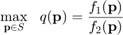
The given problem is to maximize the energy efficiency of a time invariant Gaussian channel with K parallel channel. In the paper energy efficiency (EE) is defined as the amount of data transmitted divided by the amount of energy consumed:

Since  is constant, our problem is to solve:
Proposed Solution
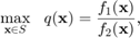
Since the problem is a ratio of two real-valued functions, the paper proposes the use of fractional programming to solve the problem. A general nonlinear fractional program has the form:
The paper presents various algorithms to solve a nonlinear fractional program for when  is concave and
  is convex. For this project I have picked and implemented only one of the proposed solutions.
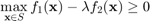
Consider the following equivalent form of the fractional program:

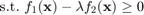
This new formulation is not jointly convex in x and  , but when is fixed, the problem will be feasible for x if
Consider the function
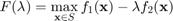
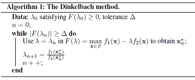
 is convex, continuous and strictly decreasing in . Solving the fractional program is equivalent to finding the root of . Which can be done with the Dinkelbach method [2]:
Data Sources
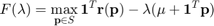
The problem to be solved is
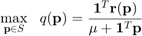
where 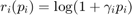 ,
,  is the channel-to-noise ratio (CNR) of subchannel
  . The
. The  for a Gaussian channel with parallel channels can be ranmdomly generated following a normal distribution and using singular-value decomposition as described in [3]:
n_t = 1; % Number of transmit antennas
n_r = 1; % Number of receive antennas
Hw = (randn(n_r, n_t) + sqrt(-1) * randn(n_r, n_t)) / sqrt(2);
[U,Lambda,V] = svd(Hw(:,:)); %singular-value decomposition
h = diag(Lambda);
No_dB = -20; %in decibel
No = 10^(No_dB/10);
gamma_value = abs(h).^2/No;
Other informations, such as  , number of transmit and receive antennas, were not given in the paper, and thus I had no way of obtaining the exact same values used in the paper. For the value of I consulted refence [4], which stated that computer models typically use something between -20 dB and 0 dB. I assumed 1 transmit antenna and 1 receive antenna, which gives us the number of subchannels K = 1.
Solution
In order to solve the problem:
It is necessary to find the root of:
Then we have from the stationary condition that:

Taking the box constraint into account,  is given by:

Now we can use the Dinkelbach method to find the root of
mu = 0.001;
tolerance = 0.00000000001; % This just needs to be a very small value
lambda_value = 0.001; % Initial lambda where F>= 0
lambda_value_next = lambda_value;
p_max = 10;
p_value = min(p_max, max(0, 1/lambda_value - 1./gamma_value));
F1 = ones(length(gamma_value),1)'*log10(1 + gamma_value.*p_value);
F2 = mu + ones(length(p_value),1)'*p_value;
F = F1 - lambda_value*F2;
% Making sure that F > 0 for the initial value of lambda
while F < 0
    % In case F < 0 with the initial lambda_value we get a smaller
    % lambda_value
    lambda_value = lambda_value/10;
    p_value = min(p_max, max(0, 1/lambda_value - 1./gamma_value));
    F1 = ones(length(gamma_value),1)'*log10(1 + gamma_value.*p_value);
    F2 = mu + ones(length(p_value),1)'*p_value;
    F = F1 - lambda_value*F2;
end
% Dinkelbach method
counter = 0;
while abs(F) >= tolerance
    lambda_value = lambda_value_next;
    p_value = min(p_max, max(0, 1/lambda_value - 1./gamma_value));
    F1 = ones(length(gamma_value),1)'*log10(1 + gamma_value.*p_value);
    F2 = mu + ones(length(p_value),1)'*p_value;
    F = F1 - lambda_value*F2;
    lambda_value_next = F1/F2;
    counter = counter + 1;
end
With the optimum  and
and  , we find the maximum
  .
.
In order to reproduce the results presented in the paper [1] we also implemented a constrained case:
lambda_max = 5; %These values were taken from Fig. 2 from [1]
lambda_min = 0.1;
lambda_constrained = 0.1;
p_constrained = min(p_max, max(0, 1/lambda_constrained - 1./gamma_value));
F1 = ones(length(gamma_value),1)'*log10(1 + gamma_value.*p_constrained);
F2 = mu + ones(length(p_constrained),1)'*p_constrained;
F = F1 - lambda_constrained*F2;
% Making sure that F > 0 for the initial value of lambda
while F < 0
    lambda_constrained = lambda_constrained/10;
    p_constrained = min(p_max, max(0, 1/lambda_constrained - 1./gamma_value));
    F1 = ones(length(gamma_value),1)'*log10(1 + gamma_value.*p_constrained);
    F2 = mu + ones(length(p_constrained),1)'*p_constrained;
    F = F1 - lambda_constrained*F2;
end
lambda_value_next = lambda_constrained;
% Dinkelbach method
counter = 0;
while abs(F) >= tolerance
    lambda_constrained = lambda_value_next;
    p_constrained = min(p_max, max(0, 1/lambda_constrained - 1./gamma_value));
    F1 = ones(length(gamma_value),1)'*log10(1 + gamma_value.*p_constrained);
    F2 = mu + ones(length(p_constrained),1)'*p_constrained;
    F = F1 - lambda_constrained*F2;
    lambda_value_next = min(lambda_max, max(lambda_min, F1/F2));
    counter = counter + 1;
    % Since we have constraints for lambda, we may never find the root of
    % F. Thus, after enough iterations we just exit the loop
    if counter > 10000
       break;
    end
end
Please find bellow the full code to obtain the maxmimum for  varying from 0.0001 to 1000.
close all;
clear all;

graph_size = 100;
mu_vector = logspace(-4,4,graph_size);
q_vector = zeros(1,graph_size);
q_constrained_vector = zeros(1,graph_size);
n_t = 1; % Number of transmit antennas
n_r = 1; % Number of receive antennas
No_dB = -20; %in decibel
No = 10^(No_dB/10);
for mu_counter = 1:graph_size
    mu = mu_vector(mu_counter);
    nsample = 10000;
    Hw = (randn(n_r, n_t, nsample) + sqrt(-1) * randn(n_r, n_t, nsample)) / sqrt(2);
    q_sum = 0;
    q_constrained_sum = 0;
    for h_counter = 1:nsample
        [U,Lambda,V] = svd(Hw(:,:,h_counter));%singular-value decomposition
        h = diag(Lambda);
        gamma_value = abs(h).^2/No;
        tolerance = 0.00000000001;
        lambda_value = 0.001;
        lambda_value_next = lambda_value;
        p_max = 10; %10
        p_value = min(p_max, max(0, 1/lambda_value - 1./gamma_value));
        F1 = ones(length(gamma_value),1)'*log10(1 + gamma_value.*p_value);
        F2 = mu + ones(length(p_value),1)'*p_value;
        F = F1 - lambda_value*F2;
        % Making sure that F > 0 for the initial value of lambda
        while F < 0
            lambda_value = lambda_value/10;
            p_value = min(p_max, max(0, 1/lambda_value - 1./gamma_value));
            F1 = ones(length(gamma_value),1)'*log10(1 + gamma_value.*p_value);
            F2 = mu + ones(length(p_value),1)'*p_value;
            F = F1 - lambda_value*F2;
        end
        % Dinkelbach method
        counter = 0;
        while abs(F) >= tolerance
            lambda_value = lambda_value_next;
            p_value = min(p_max, max(0, 1/lambda_value - 1./gamma_value));
            F1 = ones(length(gamma_value),1)'*log10(1 + gamma_value.*p_value);
            F2 = mu + ones(length(p_value),1)'*p_value;
            F = F1 - lambda_value*F2;
            lambda_value_next = F1/F2;
            counter = counter + 1;
        end
        q = ones(length(gamma_value),1)'*log10(1 + gamma_value.*p_value)/(mu + ones(length(p_value),1)'*p_value);
        q_sum = q_sum + q;
        % Constrained case
        % For when you have a maximum and minimum lambda
        lambda_max = 5;
        lambda_min = 0.1;
        lambda_constrained = 0.1;
        p_constrained = min(p_max, max(0, 1/lambda_constrained - 1./gamma_value));
        F1 = ones(length(gamma_value),1)'*log10(1 + gamma_value.*p_constrained);
        F2 = mu + ones(length(p_constrained),1)'*p_constrained;
        F = F1 - lambda_constrained*F2;
        % Making sure that F > 0 for the initial value of lambda
        while F < 0
            lambda_constrained = lambda_constrained/10;
            p_constrained = min(p_max, max(0, 1/lambda_constrained - 1./gamma_value));
            F1 = ones(length(gamma_value),1)'*log10(1 + gamma_value.*p_constrained);
            F2 = mu + ones(length(p_constrained),1)'*p_constrained;
            F = F1 - lambda_constrained*F2;
        end
        lambda_value_next = lambda_constrained;
        % Dinkelbach method
        counter = 0;
        while abs(F) >= tolerance
            lambda_constrained = lambda_value_next;
            p_constrained = min(p_max, max(0, 1/lambda_constrained - 1./gamma_value));
            F1 = ones(length(gamma_value),1)'*log10(1 + gamma_value.*p_constrained);
            F2 = mu + ones(length(p_constrained),1)'*p_constrained;
            F = F1 - lambda_constrained*F2;
            lambda_value_next = min(lambda_max, max(lambda_min, F1/F2));
            counter = counter + 1;
            if counter > 100
               break;
            end
        end
        p_constrained = min(p_max, max(0,1/lambda_constrained - 1./gamma_value));
        q_constrained = ones(length(gamma_value),1)'*log10(1 + gamma_value.*p_constrained)/(mu + ones(length(p_constrained),1)'*p_constrained);
        q_constrained_sum = q_constrained_sum + q_constrained;
    end
    q_vector(mu_counter) = q_sum/nsample;
    q_constrained_vector(mu_counter) = q_constrained_sum/nsample;
end
Visualization of results
Find bellow the code to print the resulting curves and the resulting Figure.
cc = lines(11);
figure()
loglog(mu_vector, q_vector, '-k', 'LineWidth', 1.5)
hold on
loglog(mu_vector, q_constrained_vector, '--b', 'LineWidth', 1.5)
grid on;
legend('Unconstrained solution','Constrained solution', 'Location', 'Southwest');
ylabel('q* (bit/J)');
xlabel('\mu (W)');
ylim([0.0001 100]);
hold off
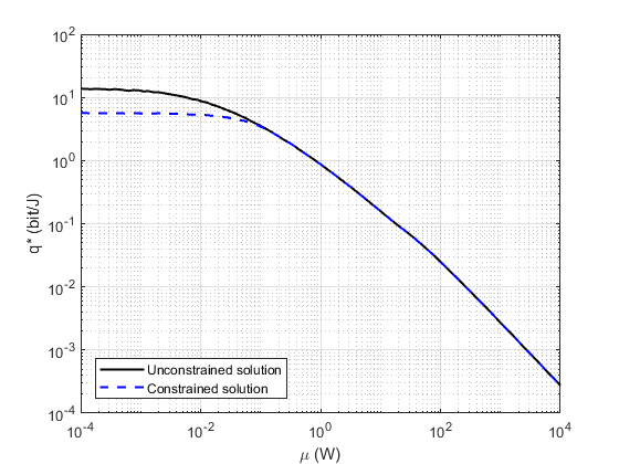
Analysis and Conclusions
In this project, I have implemented one of the many proposed solutions proposed in [1] to solve a non-linear fractional program.
The resulting Figure, although similar to Fig. 2 presented in [1], is not the same. When comparing the figures, it is possible to see, for example, that for  ,
,  is smaller on our figures than it is on fig. 2 of [1]. The difference in results is probably due to the fact that the paper did not specify the values used to obtain Fig. 2. Changing the values of , the number of receiving and transmit antennas (
 and
and  ) and
) and  can drastically change the shape of the curves.
Despite the difference in the results, I believe that I was able to correctly implement the solution presented in [1], as the implemented Dinkelbach algorithm was able to find the root of for the unconstrained case.
The solution proposed by the authors of the original paper can solve the proposed fraction non-linear program quite fast for a small number of channels, however, for K > 3 the solutions are much slower.
References and Links
[1] C. Isheden, Z. Chong, E. Jorswieck and G. Fettweis, "Framework for Link-Level Energy Efficiency Optimization with Informed Transmitter," in IEEE Transactions on Wireless Communications , vol. 11, no. 8, pp. 2946-2957, August 2012.
[2] W. Dinkelbach, "On nonlinear fractional programming," Management Science, vol. 13, no. 7, pp. 492-498, Mar. 1967.
[3] D. Tse and P. Viswanath, Fundamentals of Wireless Communication , 2006.
[4] https://www.mathworks.com/help/comm/ug/fading-channels.html