ADAM: A METHOD FOR STOCHASTIC OPTIMIZATION
Xiaotong Chen 20713364
Valerie McKay-Crites 20732319
ECE 602 - Winter 2018
Prof. Oleg Michailovich
Paper: ADAM: A Method for Stochastic Optimization by Diederik P. Kingma and Jimmy Lei Ba [1]
Contents
Problem formulation
The authors propose ADAM, a simple and computationally efficient method for gradient-based optimization of stochastic objective functions. It combines the advantages of two recently popular optimization methods: the ability of AdaGrad to deal with sparse gradients, and the ability of RMSProp to deal with non-stationary objectives. The project evaluated the method on multi-class logistic regression using the MNIST dataset.
Proposed Solution
1. Adam algorithm
Adam update rule consists of the following steps:
- Compute gradient
 at current time
  .
.
- Update biased first moment estimate.

It is computing a moving average of the derivatives for parameters. The gradient descent with momentum ends up taking steps that produce much smaller oscillations. This allows the algorithm to take a more straightforward path to the minimum. One of the advantages of this exponentially weighted average formula is that it takes very little memory. We need to keep just one row number in computer memory. The formula keeps on overwriting old values with the latest values. It is really efficient compared with the average over all parameters, as it only takes one line of code , and the storage for the memory of a single raw number.
- Update biased second raw moment estimate.
We want the learning rate to be fast to converge, and we want to slow down the oscillations. So, with the term  , what we're hoping is that it will be relatively small. Parameters that gets few or small updates receive higher learning rates. One effect is that we can use a larger learning rate that decreases over time, and get faster learning without diverging in the vertical direction.
- Compute bias-corrected first moment estimate.

- Compute bias-corrected second raw moment estimate.

When we are implementing a moving average, the initialization value of  is zero. Then the first several values of are lower. It is not a very good estimate of the gradients. Bias-corrected first momentum is a way to modify this estimate to make it more accurate, especially during this initial phase of the estimate.
  will remove the bias. As iteration is low, the denominator is low and becomes larger.
- Update parameters.
2. Logistic Regression
minimize 
where  is the variable, and
  is the logistic loss
where  is the number of training data
  , and
, and 
The multiclass classification is to choose the maximum value among binary classifiers for single input data corresponds to the output class label and can be expressed as follows:

where  is the number of the binary classifiers corresponding to the number of classes
- Gradients:
For i = 1 to m, j = 1 to n

where m is the number of samples and n is the number of dimensions.
- Update parameters
 using gradient with Adam
Data sources
We take the MNIST dataset training image files [3] and convert them to matlab files. We use the labels file as a categorical and the images training file as a double vector. We use the 60000 MNIST images as training set and convert them to 784-d vectors. Then the samples are randomly split into different mini-batches (size 128 except last one is 95). Mini-batches require less computation to update the weights.
clear; clc;

load IMAGES.mat
load LABELS.mat

% Create a shuffled version of the training set
p = randperm(size(IMAGES,1));
I_shuffle = zeros(60000,784);
labels_shuffle= categorical(zeros(60000,1));
for i = 1:size(I_shuffle,1)
     I_shuffle(i,:) = IMAGES(p(i),:);
     labels_shuffle(i,1) = LABELS(p(i));
end
% Create mini-batches
for j = 1:468
    I(j).image = I_shuffle(128*j-127:128*j,:);
    I(j).labels = labels_shuffle(128*j-127:128*j,:);
end
I(469).image = I_shuffle(59905:60000,:);
I(469).labels = labels_shuffle(59905:60000,:);
Solution
ADAM
% initialize variables
N = 784;
w = randn(N,10) * 0.01; b = randn(10,1) * 0.01;
V_dw = zeros(N,10); V_db = zeros(10,1);
S_dw = zeros(N, 10); S_db = zeros(10,1);
% Hyperparameters
iter = 45;
alpha = 0.01;
belta1 = 0.9;
belta2 = 0.999;
epsilon = 10.^(-8);
batches=469;
cost = zeros(batches,iter);
cost1 = zeros(1,iter);
for k = 1:iter
       for i = 1:batches
         % Forward Propagation
         a = forward_propagation(I(i).image, w, b);

         % Compute cost
         cost(i,k) = compute_cost(a, I(i).labels);

         % Backward propagation
         [dw, db] = backward_propagation(I(i).image, I(i).labels, a);

         %Update Parameters with Adam
         [w, b, V_dw, V_db, S_dw, S_db] = update_parameters_adam(I(i).image,...
           dw, db, w, b, V_dw, V_db, S_dw, S_db, alpha, belta1, belta2, k, epsilon);

       end
       cost1(k) = cost(k,k);
        if mod(k-1,5) == 0 || k > 40
            if k == 1
                fprintf('ADAM Values Every 5 Iterations \n');
            end
            fprintf('Cost for ADAM after iteration %d: %f \n', k-1, cost(k,k));
       end
end
AdaGrad
In this experiment, the paper compares Adam with two different optimizers: AdaGrad and SGD with Nesterov momentum.
AdaGrad is a modified stochastic gradient descent with per-parameter learning rate [2]. It increases the learning rate for more sparse parameters and decreases the rate for less sparse ones.
where  is the gradient at iteration . This vector is updated after every iteration. The formula for an update is
AdaGrad corresponds to a version of Adam with  , infinitesimal
  and a replacement of
  by an annealed version
  . Therefore, we could implement AdaGrad by changing Adam algorithm.
% initialize variables
N = 784;
w = randn(N,10) * 0.01; b = randn(10,1) * 0.01;
V_dw = zeros(N,10); V_db = zeros(10,1);
S_dw = zeros(N, 10); S_db = zeros(10,1);
% Hyperparameters
iter = 45;
batches = 469;
alpha = 0.01;
% Changing hyperparameters
belta1 = 0;
belta2 = 0.999999;
epsilon = 10.^(-8);
cost2 = zeros(1,iter);
for k = 1:iter
       for i = 1:batches

         % Forward Propagation
         a = forward_propagation(I(i).image, w, b);

         % Compute cost
         cost(i,k) = compute_cost(a, I(i).labels);

         % Backward propagation
         [dw, db] = backward_propagation(I(i).image, I(i).labels, a);

         % Update Parameters with AdaGrad
         [w, b, V_dw, V_db, S_dw, S_db] = update_parameters_AdaGrad(I(i).image,...
           dw, db, w, b, V_dw, V_db, S_dw, S_db, alpha, belta1, belta2, k, epsilon);

       end
       cost2(k) = cost(k,k);
end
SGD Nesterov
First make a big jump in the direction of the previous accumulated gradient. Then measure the gradient where we end up and make a correction.
% initialize variables
N = 784;
w = randn(N,10) * 0.01; b = randn(10,1) * 0.01;
V_dw = zeros(N,10); V_db = zeros(10,1);
S_dw = zeros(N, 10); S_db = zeros(10,1);
% Hyperparameters
iter = 45;
batches = 469;
alpha = 0.1;
belta1 = 0.9;
belta2 = 0.999;
epsilon = 10.^(-8);
cost = zeros(batches,iter);
cost3 = zeros(1,iter);
for k = 1:iter
       for i = 1:batches

         % Forward Propagation
         a = forward_propagation(I(i).image, w, b);

         % Compute cost
         cost(i,k) = compute_cost(a, I(i).labels);

         % Backward propagation
         [dw, db] = backward_propagation(I(i).image, I(i).labels, a);

        % Update Parameters with SGDNesterov
        [w, b, V_dw, V_db] = update_parameters_SGDNesterov(I(i).image, dw, db, w, b,...
            V_dw, V_db, alpha, belta1, k);
       end
       cost3(k) = cost(k,k);
end
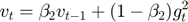
Visualization of results
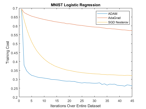
figure, plot(cost1);
hold on, plot(cost2);
hold on, plot(cost3);
axis([0 45 0.2 0.7]);
legend('ADAM', 'AdaGrad', 'SGD Nesterov');
title('MNIST Logistic Regression');
xlabel('Iterations Over Entire Dataset');
ylabel('Training Cost')
%
% The random fluctuations in the error due to the different gradients on
% different mini-batches.
Solvers and Functions
- compute_cost
- forward_propagation
- backward_propagation
- update_parameters_adam
- update_parameters_AdaGrad
- update_parameters_SGDNesterov
function cost = compute_cost(a, labels)
cost = 0;
      for i = 1:size(labels,1)
        num = str2num(char(labels(i)));
        y = zeros(10,1);
        y(num+1) = 1;
        % Cost Function
        cost = cost + ( -( y' * log( a(i, :)' ) + ( 1 - y )' * log( 1 - a(i, :)')) )  /size(labels,1)/10;
      end
end
%%%%%%%%%%%%%%%%%%%%%%%%%%%%%%%%%%%%%%%%%%%%%%%%%%%%%%%%%%%%%%%%%%%%%%%%%%%%%%%%
%%%%%%%%%%%%%%%%%%%%%%%%%%%%%%%%%%%%%%%%%%%%%%%%%%%%%%%%%%%%%%%%%%%%%%%%%%%%%%%%
function a = forward_propagation(I, w, b)
z= zeros( size(I,1), 10);
a = zeros( size(I,1), 10);
    for i = 1:size(I,1)
        for j = 1:size(w,2)
            % Output of Logistic Regression
            z(i,j) = w(:,j)' * I(i,:)'./255 + b(j);
            a(i,j) = 1./(1+exp(-z(i,j)));
        end
    end
end
%%%%%%%%%%%%%%%%%%%%%%%%%%%%%%%%%%%%%%%%%%%%%%%%%%%%%%%%%%%%%%%%%%%%%%%%%%%%%%%%
%%%%%%%%%%%%%%%%%%%%%%%%%%%%%%%%%%%%%%%%%%%%%%%%%%%%%%%%%%%%%%%%%%%%%%%%%%%%%%%%
function [dw, db] = backward_propagation(I, labels, a)
dw = zeros(size(I,2),10); db = zeros(10,1);
y = zeros(10, size(a,1));
    for i=1:size(I,1)
        num(i) = str2num(char(labels(i)));
        y(num(i)+1, i) = 1;
    end
dz = a' - y;
db = sum(dz,2) ./ size(I,1);
dw = I' * dz' ./ size(I,1);
end
%%%%%%%%%%%%%%%%%%%%%%%%%%%%%%%%%%%%%%%%%%%%%%%%%%%%%%%%%%%%%%%%%%%%%%%%%%%%%%%%
%%%%%%%%%%%%%%%%%%%%%%%%%%%%%%%%%%%%%%%%%%%%%%%%%%%%%%%%%%%%%%%%%%%%%%%%%%%%%%%%
function [w, b, V_dw, V_db, S_dw, S_db] = update_parameters_adam(I, dw, db, w, b, V_dw, V_db, S_dw, S_db, alpha, belta1, belta2, t, epsilon)

    % Momentum
    V_dw = belta1 .* V_dw + (1-belta1) * 1/size(I,1) .* dw;
    V_db = belta1 .* V_db + (1-belta1) * 1/size(I,1) .* db;

    % RMSprop
    S_dw = belta2 .* S_dw + (1-belta2) * 1/size(I,1) .* dw.^2;
    S_db = belta2 .* S_db + (1-belta2) * 1/size(I,1) .* db.^2;

    alpha = alpha/sqrt(t);

    w = w - alpha .* V_dw ./ (sqrt(S_dw) + epsilon);
    b = b - alpha .* V_db ./ (sqrt(S_db) + epsilon);
end
%%%%%%%%%%%%%%%%%%%%%%%%%%%%%%%%%%%%%%%%%%%%%%%%%%%%%%%%%%%%%%%%%%%%%%%%%%%%%%%%
%%%%%%%%%%%%%%%%%%%%%%%%%%%%%%%%%%%%%%%%%%%%%%%%%%%%%%%%%%%%%%%%%%%%%%%%%%%%%%%%
function [w, b, V_dw, V_db, S_dw, S_db] = update_parameters_AdaGrad(I, dw, db, w, b, V_dw, V_db, S_dw, S_db, alpha, belta1, belta2, t, epsilon)

    % Calculate an exponentially weighted average of past gradients, and
    % stores it in variables v.
    V_dw = belta1 .* V_dw + (1-belta1) * 1/size(I,1) .* dw;
    V_db = belta1 .* V_db + (1-belta1) * 1/size(I,1) .* db;

    % Calculate an exponentially weighted average of the squares of past
    % gradients, and stores it in variables S
    S_dw = belta2 .* S_dw + (1-belta2) * 1/size(I,1) .* dw.^2;
    S_db = belta2 .* S_db + (1-belta2) * 1/size(I,1) .* db.^2;

    % Bias-Correct
    V_dw_corrected = V_dw./ (1-belta1^t);
    V_db_corrected = V_db ./ (1-belta1^t);

    S_dw_corrected = S_dw./ (1-belta2^t);
    S_db_corrected = S_db ./ (1-belta2^t);

    % Update parameters in a direction based on v and S
    w = w - alpha/sqrt(t) .* V_dw_corrected ./ (sqrt(S_dw_corrected) + epsilon);
    b = b - alpha/sqrt(t) .* V_db_corrected ./ (sqrt(S_db_corrected) + epsilon);

end
%%%%%%%%%%%%%%%%%%%%%%%%%%%%%%%%%%%%%%%%%%%%%%%%%%%%%%%%%%%%%%%%%%%%%%%%%%%%%%%%
%%%%%%%%%%%%%%%%%%%%%%%%%%%%%%%%%%%%%%%%%%%%%%%%%%%%%%%%%%%%%%%%%%%%%%%%%%%%%%%%
function [w, b, V_dw, V_db] = update_parameters_SGDNesterov(I, dw, db, w, b, V_dw, V_db, alpha, belta1, t)
    % Momentum
    V_dw = belta1 .* V_dw + (1-belta1) * 1/size(I,1) .* dw;
    V_db = belta1 .* V_db + (1-belta1) * 1/size(I,1) .* db;

    w = w - alpha .* V_dw;
    b = b - alpha .*  V_db;
end
%%%%%%%%%%%%%%%%%%%%%%%%%%%%%%%%%%%%%%%%%%%%%%%%%%%%%%%%%%%%%%%%%%%%%%%%%%%%%%%%
ADAM Values Every 5 Iterations
Cost for ADAM after iteration 0: 0.694234
Cost for ADAM after iteration 5: 0.318023
Cost for ADAM after iteration 10: 0.304476
Cost for ADAM after iteration 15: 0.295369
Cost for ADAM after iteration 20: 0.287921
Cost for ADAM after iteration 25: 0.281101
Cost for ADAM after iteration 30: 0.277861
Cost for ADAM after iteration 35: 0.272720
Cost for ADAM after iteration 40: 0.264486
Cost for ADAM after iteration 41: 0.261258
Cost for ADAM after iteration 42: 0.268538
Cost for ADAM after iteration 43: 0.266488
Cost for ADAM after iteration 44: 0.262349
Analysis and conclusions
Adam is an optimization algorithm that can used instead of the classical stochastic gradient descent procedure to update network weights iteratively based on training data. There are attractive benefits of using Adam as follows:
- Straightforward to implement.
- Computationally efficient.
- Little memory requirements.
- Well suited for problems that are large in terms of data.
- Appropriate for non-stationary objectives.
- Appropriate for problems with very sparse gradients.
- Hyper-parameters have intuitive interpretation and typically require little tuning.
In reproducing the results of the paper "ADAM: A Method for Stochastic Optimization", we found our algorithm for ADAM had very similar results. Our implementation converges similarly to the SGD Nesterov method for the MNIST dataset. As well we also observed that both of those methods converge faster than ADAGrad for the MNIST database.
References
[1] Kingma, D.P. and Ba, J., 2014. Adam: A method for stochastic optimization. arXiv preprint arXiv:1412.6980.
[2] Duchi, J., Hazan, E. and Singer, Y., 2011. Adaptive subgradient methods for online learning and stochastic optimization. Journal of Machine Learning Research, 12(Jul), pp.2121-2159.
[3] Y. LeCun, C. Cortes and C. Burges, "MNIST handwritten digit database", Yann.lecun.com, 2010. [Online]. Available: http://yann.lecun.com/exdb/mnist/. [Accessed: 14- Apr- 2018].