Fast trigonometric functions
Libraries implementing trigonometric functions will, on occasion, use strategies
such as storing a fixed number of points and then using some form of interpolation.
For example, one digital signal processing library divides the interval
into 256 intervals and expects the
user to pass in a value of
. The techniques used include
- linear interpolation using the two neighboring, and
- cubic interpolation using four neighboring points.
First, in order to make this more reasonable, it would make sense to restrict the
domain of the function to the interval , as up to
a sign difference, this contains all values. Dividing this interval into 256 sub-intervals
(with 257 points), we note that the maximum error is given in the following table:
| Linear interpolation | |
| Cubic interpolation |
I will attempt to argue that in both cases, the algorithms used are sub-optimal and equally fast algorithms are available that run in approximately the same time requiring in one case an allocation of memory.
Using the binary representation
If the user passes a value on the interval to represent a scaled value
on the range
, we can use the floating-point representation very
effectively:
- For any number
, calculate the value
.
- For any number
, calculate the value
.
- For any number
, calculate the value
.
- For any number
, calculate the value
.
This will leave one special case: for , return
.
Having dealt with the special case, we must now approximate the trigonometric function at the value .
We will now assume that we have 256 = 28 intervals on which we approximate the trigonometric function. We can trivially find the interval
and the offset into the interval by taking the next 8 bits (this is the interval) and the subsequent bits (this is the offset into that interval).
Thus, given
, the bin is
and the offset into
that bin is
.
Note that we can find the bin and the offset by calculating:
	float tmp = 256 * f;

	int bin = (int) floor( f );
	double offset = frac( f );    // The factional part of the floating-point number
The latter will give a relative offset on the interval .
Requirements
In approximating a trigonometric function, the following requirements are considered to be absolutely necessary:
- The approximation must be continuous,
- If the value of the trigonometric function is 0, the approximation at that point must also be 0,
- If the value of the trigonometric function is 1, the approximation at that point must also be 1, and
- The approximation of the trigonometric function must be bounded by
.
Each of these constraints will leave unchanged or increase the error of any approximation method. Specifically, once we begin to look at using the roots of Chebyshev polynomials to define the interpolation points, this will necessarily result in interpolating polynomials that do not satisfy the end-points. We will, later, use such interpolating polynomials.
Question: what are we trying to minimize? the absolute error or the mean-squared error. The choice of interpolating polynomials will be affected by this decision.
Quadratic interpolation
Currently, one array is used to store 256 points to store just the values at the end points. It is, however, possible to pre-compute optimal quadratic functions that:
- Equal the value of the trigonometric functions at the end points, and
- Minimize the maximum absolute error on each interval.
These must be pre-computed, as there is no formula that immediately gives the coefficients
of these interpolating quadratics.
In the source directory, there is a function Fast_trig.c that stores
the coefficients of these optimal interpolating quadratic
polynomials for each interval. Consequently,
using Horner's rule, this reduces the number of operations to
- Three look-ups,
- Two multiplications, and
- Two additions.
The maximum absolute error is now reduced by a factor of almost 2500 over the
use of linear interpolating and the error is down to
. This is, however, still a factor of 50 worse
than using the interpolation strategy used by interpolating four surrounding points.
Updating the table, we now have
| Linear interpolation | |
| Quadratic interpolation | |
| Cubic interpolation |
Increasing interval width with quadratic interpolation
The significant reduction in absolute error incurred by switching from linear interpolation
to quadratic interpolation includes a significant increase in memory use. Consequently, to
demonstrate the robustness of the algorithm,
a second example uses only 64 intervals; thereby the three
arrays require only 75 % of the memory than the original array of 256 entries.
The maximum absolute
error, however, is still lower: , still a reduction in
error by a factor of almost 40 over linear interpolation.
Updating the table, we have
| Linear interpolation | |
| Quadratic interpolation (64 points) | |
| Quadratic interpolation (256 points) | |
| Cubic interpolation |
The left-hand menu has a source directory that implements both the 256- and 64-point optimized quadratic polynomial interpolating functions. It should be noted that the optimized quadratic polynomials were found using the symbolic computation package Maple.
Derivative matching cubic interpolating polynomials
One significant issue when using cubic polynomials spanning four points to approximate values between the inner two points is that the interpolating quadratic functions have derivatives that already vary at the two end-points. Consequently, the piecewise interpolating polynomials match at the endpoints of the intervals on which they approximate the solution; however, the derivatives do not even match—sub-optimal at best if continuous differentiability at these points is desired.
This technique is reduced to using the following four constraints to find the coefficients of the cubic polynomial:
Another means of defining four constraints is to find the interpolating polynomial that matches the both values and the derivatives at the two interior points:
Because look-up tables exist for both trigonometric functions (or could be easily deduced
from one table), this requires no additional memory. The maximum absolute error is
now reduced to , a reduction by a factor of 9 over using
the interpolating polynomial using four surrounding points—with no additional work
required.
Updating the table, we have
| Linear interpolation | |
| Quadratic interpolation (64 points) | |
| Quadratic interpolation (256 points) | |
| 4-point cubic interpolation | |
| 2-point derivative-matching cubic interpolation |
Consequently, if the interpolating cubic polynomials are to be calculated dynamically based on only two tables, it is recommended that the 2-point derivative-matching interpolating cubics be used; while for the faster version, it is recommended that pre-calculated optimal quadratic be stored using 64 points, yielding a reduction in error, equivalent speed, and a reduction in memory.
Optimized cubic interpolating polynomials
If we do not constrain ourselves to matching the derivatives at the end, but rather only matching the end-points, we can reduce the error further. As in the quadratic case, two sets of optimized cubic polynomials: one using 256 intervals and one using 64 intervals. As the coefficient array is now the same, the 64-interval algorithm now occupies as much memory as the previous. The error, however, is still reduced, as is shown in the following table and the code is implemented in the source directory in the left-hand column.
| Linear interpolation | |
| Quadratic interpolation (64 points) | |
| Quadratic interpolation (256 points) | |
| Optimized cubic interpolation (64 points) | |
| 4-point cubic interpolation | |
| 2-point derivative-matching cubic interpolation | |
| Optimized cubic interpolation (256 points) |
Thus, using optimized cubic interpolation with 64 points is worse than the method finding an interpolating polynomial matching four surrounding points; however, as Horner's rule need only be applied, it is significantly faster. The optimized cubic interpolation is better than quadratic interpolation; however, the question is whether the additional memory is worth the reduction in error by a factor of three and the reduction in the number of multiplications and additions to each (in each case, reducing the number of computations by a factor of three).
Removing the last constraint
The last constraint we have is that the interpolating polynomials actually match the value of the sine function at the 257 or 65 points. If we remove this restriction and only require that the interpolating polynomials are continuous, the error could be reduced by a further factor of probably two. This, however, would require us to solve a system of equations while iterating to a solution.
Linear Interpolating Function using Chebyshev Polynomials
An interpolating function that uses the roots of the nth Chebyshev polynomial minimizes the
absolute error of a polynomial of degree n - 1 interpolating a polynomial of degree n.
For a linear interpolating function, this means using points relative to
on the interval
. In this case, however, we have three issues that plague us:
- The interpolating functions no longer form a continuous function,
- The interpolating function is not 0 at 0 for the sine function,
- The interpolating function is not 1 at
, and
- The interpolating function exceeds 1 around the maximum.
In order to fix this, we do the following change:
- The first and last interpolating polynomials are fixed to pass through the end points. (This
means we must use the points
relative to the interval
to find the interpolating polynomial that minimize the maximum error but also passes through the right-hand end point.)
- For each point were the polynomials meet, we will add a correction factor in terms of a linear polynomial on each interval which makes both line up.
This also solves the issue that the interpolating polynomials exceed the value of 1. This is implemented in the function linear_chebyshev_sin_256 in the source directory. The issue with this interpolating function is that the error on the last interval is approximately 50 % larger than the error for the entire interval;consequently, while the error is less than that of linearly interpolating 257 fixed points, one cannot claim the lower error globally. Consequently, it may be better if a different interpolating (quadratic?) was used on the last interval. The updated error table is now:
| Linear interpolation | |
| Linear interpolation with Chebyshev roots (256 points) | |
| Linear interpolation with Chebyshev roots w/alternate strategy on last interval (256 points) | |
| Quadratic interpolation (64 points) | |
| Quadratic interpolation (256 points) | |
| Optimized cubic interpolation (64 points) | |
| 4-point cubic interpolation | |
| 2-point derivative-matching cubic interpolation | |
| Optimized cubic interpolation (256 points) |
An alternate technique is to iteratively find the optimal polynomial: at each endpoint, find that linear polynomial that passes through (0, 0) and (π, 1) and minimizes the absolute error. Then, taking these as starting points, find the linear polynomial that passes through the endpoints and which minimizes the absolute error on the next interval, and iterate. This process is continued until polynomials are found through all intervals and a correction is made at the end where the two iterations meet. This is described as optimized linear interpolation.
Actual Error
The actual errors are shown in Figures 1 through 5. You will note that for the optimal interpolating quadratics, the error is both positive and negative, but due to the nature of higher derivatives of the trigonometric function on the interval, the other errors are strictly positive.
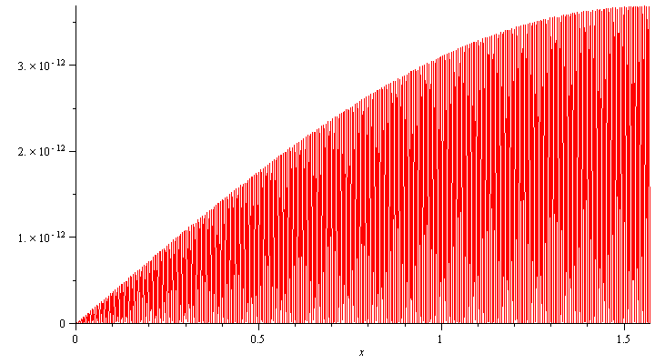
Figure 1. Error in approximating values on the interval
using cubic polynomials matching the values and derivatives at two surrounding points chosen
from 256 points.
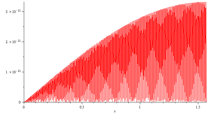
Figure 2. Error in approximating values on the interval
using cubic polynomials matching the values at four surrounding points chosen
from 256 points.
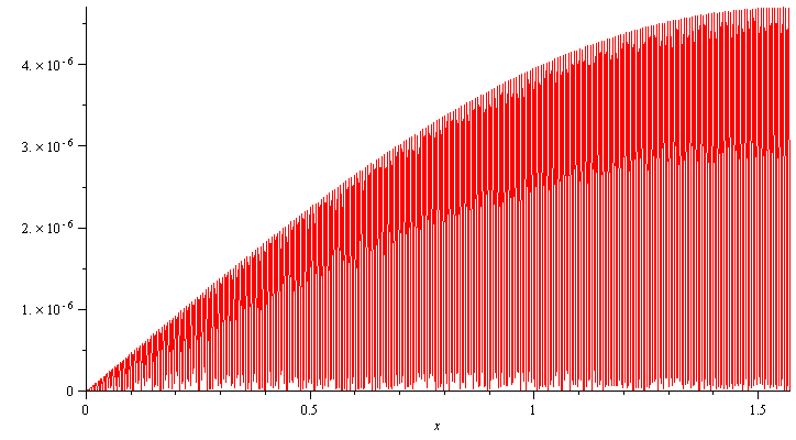
Figure 3. Error in approximating values on the interval
using linear interpolating between the two surrounding points chosen
from 256 points.
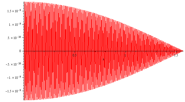
Figure 4. Error in approximating values on the interval
using optimized quadratic polynomials matching the values at two surrounding points chosen
from 256 points.
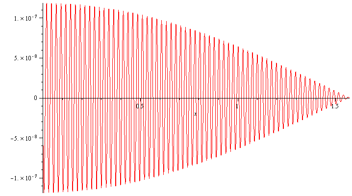
Figure 5. Error in approximating values on the interval
using optimized quadratic polynomials matching the values at two surrounding points chosen
from 64 points.
