Given a curve, a secant line (or just secant) is a line which passes through two points of that curve. To understand why the secant function is so named, see trigonometric functions.
The secant method is a technique for finding the root of a scalar-valued function f(x) of a single variable x when no information about the derivative exists. It is similar in many ways to the false-position method, but trades the possibility of non-convergence for faster convergence.
Background
Useful background for this topic includes:
- 3. Iteration
- 5. Interpolation
References
- Bradie, Section 2.5, Secant Method, p.107.
- Mathews, Section 2.4, Newton-Raphson and Secant Methods, p.80.
- Weisstein, http://mathworld.wolfram.com/SecantMethod.html.
Theory
Assumptions
If we do not have the derivative of the function, we must resort to interpolation when trying to find a root.
We will assume that f(x) is a real-valued function of a single variable x.
Derivation
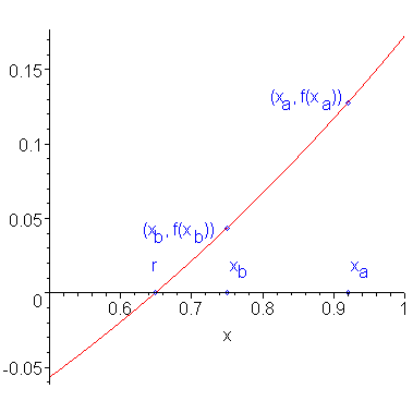
Suppose we have two approximations xa and xb to a root r of f(x), that is, f(r) = 0. Figure 1 shows a function with a root and an approximation to that root.

Figure 1. A function f(x), a root r, and an approximation to that root xa.
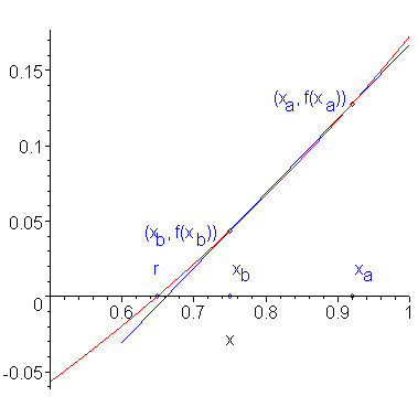
Because f(x) is continuous, and in this case, differentiable, we could approximate the function by interpolating the two points (xa, f(xa)) and (xb, f(xb)). This interpolating line is shown in Figure 2.

Figure 1. The line tangent to the point (xa, f(xa)).
The formula for this line may be deduced quite easily: using Lagrange, the interpolating polynomial is:
Finding the root of this line is simply a matter of equating the above line to zero and solving for x:
Multiplying through by b - a, we get:
and solving for x, we get:
Thus, this value of x should be a better approximation of the root than either xa or xb.
Comment
You should recognize this as the same formula we used for the false-position method. Note, however, that an approximation of the derivative at xb is given by (f(xb) - f(xa))/(xb - xa), and therefore, with a little algebra, the above equation can be written as:
which is similar to Newton's, but using an approximation of the derivative, rather than the exact value of the derivative.
HOWTO
Problem
Given a function of one variable, f(x), find a value r (called a root) such that f(r) = 0.
Assumptions
We will assume that the function f(x) is continuous and for the technique to converge, it is useful that the function is also differentiable, but this is only necessary for the error analysis.
Tools
We will use sampling, interpolation, and iteration.
Initial Requirements
We have two initial approximation x0 and x1 of the root. It would be useful if |f(x0)| > |f(x1)|, that is, the second point is a better approximation of the root.
Iteration Process
Given the approximations xn − 1 and xn, the next approximation xn + 1 is defined to be
Halting Conditions
There are three conditions which may cause the iteration process to halt (these are the same as the halting conditions for Newton's method):
- We halt if both of the following conditions are met:
- The step between successive iterates is sufficiently small, |xn + 1 - xn| < εstep, and
- The function evaluated at the point xn + 1 is sufficiently small, |f(xn + 1)| < εabs.
- If the denominator is zero, in which case the iteration process fails (division-by-zero) and we halt.
- If we have iterated some maximum number of times, say N, and have not met Condition 1, we halt and indicate that a solution was not found.
If we halt due to Condition 1, we state that xn + 1 is our approximation to the root.
If we halt due to either Condition 2 or 3, we may either choose a different initial approximations x0 and x1, or state that a solution may not exist.
Examples
Example 1
As an example of the secant method, suppose we wish to find a root of the function f(x) = cos(x) + 2 sin(x) + x2. A closed form solution for x does not exist so we must use a numerical technique. We will use x0 = 0 and x1 = -0.1 as our initial approximations. We will let the two values εstep = 0.001 and εabs = 0.001 and we will halt after a maximum of N = 100 iterations.
We will use four decimal digit arithmetic to find a solution and the resulting iteration is shown in Table 1.
Table 1. The secant method applied to f(x) = cos(x) + 2 sin(x) + x2.
| n | xn − 1 | xn | xn + 1 | |f(xn + 1)| | |xn + 1 - xn| |
|---|---|---|---|---|---|
| 1 | 0.0 | -0.1 | -0.5136 | 0.1522 | 0.4136 |
| 2 | -0.1 | -0.5136 | -0.6100 | 0.0457 | 0.0964 |
| 3 | -0.5136 | -0.6100 | -0.6514 | 0.0065 | 0.0414 |
| 4 | -0.6100 | -0.6514 | -0.6582 | 0.0013 | 0.0068 |
| 5 | -0.6514 | -0.6582 | -0.6598 | 0.0006 | 0.0016 |
| 6 | -0.6582 | -0.6598 | -0.6595 | 0.0002 | 0.0003 |
Thus, with the last step, both halting conditions are met, and therefore, after six iterations, our approximation to the root is -0.6595 .
Engineering
To be completed...
Error
The error analysis for the secant method much more complex than that for the false-position method, because both end points are continuously being updated, and therefore, the iterations will not fall into the O(h) trap of the false-position method. It can be shown (but beyond the scope of this course) that the rate of convergence at a simple root is better than linear, but poorer than the quadratic convergence of Newton's method (Pizer, 1975) and is given by the golden-ratio

