Assumptions
We will assume that f(x) is a scalar-valued function of a single variable x and, for error analysis, that f(x) has a continuous 2nd derivative f(2)(x) which we can compute.
Derivation
We cannot reduce the error of the trapezoidal rule by changing (b - a) because this would require us to change the interval over which we are integrating. Therefore, instead, break up the interval [a, b] into n equally sized sub-intervals and apply the trapezoid rule to each of these subintervals.
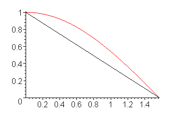
For example, Figure 1 shows a single application of the trapezoidal rule.

Figure 1. The integral of cos(x) on [0, π/2] approximated with one trapezoid.
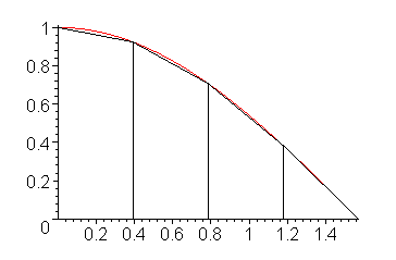
Figure 2 shows the trapezoidal rule applied to four sub-intervals on the interval [0, π/2]. It should be quite obvious that the sum of the area of the four trapezoids is a much better approximation to the integral than is the area under a single trapezoid shown in Figure 1.

Figure 2. The integral of cos(x) on [0, π/2] approximated with four trapezoids.
Thus, suppose we divide the interval [a, b] into n sub-intervals, where h = (b - a)/n. Thus, the trapezoidal rule applied to the ith interval is
where i = 1, 2, ..., n. By adding these n areas together we get
Notice that every term except for the first and last is duplicated, and the last term f(a + nh) = f(b). Thus, by factoring out ½ and h, we get the approximation
Copyright ©2005 by Douglas Wilhelm Harder. All rights reserved.


