Example 1
Apply the modified Euler-Heun method to approximate the solution to a similar IVP as shown in the theory section but with a ½(1 - cos(t)) forcing function instead of the normal curve, i.e.,
y(0) = 1
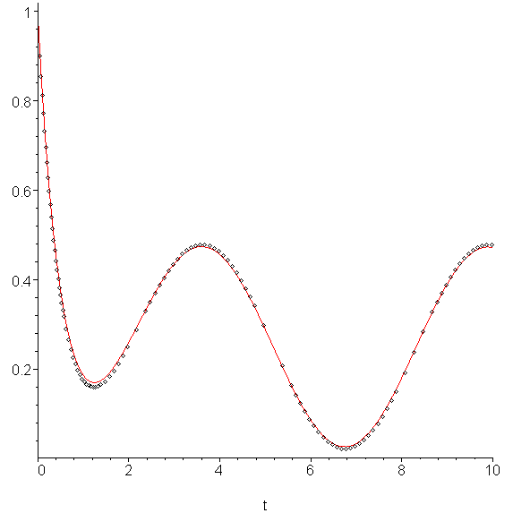
The result is as is shown in Figure 1.

Figure 1. The approximation of the given IVP in Example 1.
Example 2
Apply the modified Runge-Kutta-Fehlberg method to the IVP described in Example 1 and list the points.
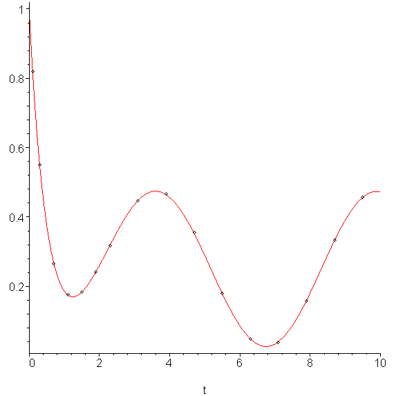
The result is as is shown in Figure 2.

Figure 2. The approximation of the given IVP in Example 1 using RKF 45.
The t values are
0, 0.1, 0.3, 0.7, 1.1, 1.5, 1.9, 2.3, 3.1, 3.9, 4.7, 5.5, 6.3, 7.1, 7.9, 8.7, 9.5, 10.3
while the actual points are
(0.3, 0.55074)
(0.7, 0.26644)
(1.1, 0.17502)
(1.5, 0.18311)
(1.9, 0.24110)
(2.3, 0.31813)
(3.1, 0.44780)
(3.9, 0.46587)
(4.7, 0.35442)
(5.5, 0.17988)
(6.3, 0.04790)
(7.1, 0.03853)
(7.9, 0.15743)
(8.7, 0.33248)
(9.5, 0.45750)
(10.3, 0.45666)
Example 3
Approximate y(π) and y(5) using the points in Example 2.
Because π ≈ 3.1, we can probably interpolate the three points around 3.1 and evaluate the quadratic at π.
Using Matlab:
>> x = [2.3 3.1 3.9]';
>> y = [0.31813 0.44780 0.46587]';
>> poly = vander( x ) \ y
ans =

  -0.08719
   0.63290
  -0.67632

>> polyval( poly, pi )
ans = 0.45149
Because 5 is closer to the mid point between 4.7 and 5.5, it is probably best to find the interpolating cubic.
>> x = [3.9 4.7 5.5 6.3]';
>> y = [0.46587 0.35442 0.17988 0.04790]';
>> poly = vander( x ) \ y
poly =

   0.03439
  -0.53421
   2.54167
  -3.36144

>> polyval( poly, 5 )
ans = 0.29069
Example 4
Given that the actual solution to the IVP given in Example 1is the function
what is the relative error of the two values found in Example 3. Which is better and why?
From the function, we get that y(π) = (9 + 19e-2π)/20 ≈ 0.4517740706, and therefore the relative error is 0.000629.
From the function, we get that y(5) ≈ 0.2892031203, and therefore the relative error is 0.00514.
The relative error of the first is smaller because the point π was closer to one of the actual points, namely, 3.1. As you move away from the interpolating points, the error increases.
Copyright ©2006 by Douglas Wilhelm Harder. All rights reserved.


