Introduction Notes Theory HOWTO Examples Engineering Error Questions Matlab Maple

The trapezoidal rule ½(f(a) + f(b))(b - a) for integration is much better than using only the left end-point with a formula like f(a)(b - a) because it samples the value of the function at two points. If the function is reasonably smooth, then the interpolation of these two points is appropriate. Similarly, Euler's method only samples the slope at the left end-point, that is, the initial point (t₀, y₀). Heun's method is an attempt to use information about the slope at both end points to find the average slope.

Like Euler, the eu in Heun sounds like oi, that is, Heun rhymes with coin.

Background

Useful background for this topic includes:

7. Taylor Series
14.1 Euler's Method

References

Bradie, Section 7.4, Runge-Kutta Methods, p.572.
Mathews, Section 9.3, Heun's Method, p.465.

Interactive Maplet

A Demonstration of Heun's Method

Theory

Euler's method only samples the slope at the left end-point, that is, the initial point (t₀, y₀). Let's call this first slope K₀ = f(t₀, y₀). Then if h = t₁ - t₀, then y₁ = y₀ + h K₀ is Euler's approximation of y(t₁).

Let's now sample the slope at this new point (t₁, y₁), that is, K₁ = f(t₁, y₁). This is only an approximation of the actual slope at y(t₁) because y₁ is only an approximation of y(t₁). Thus, K₁ is not as accurate as K₀, but let us assume it is still a reasonable approximation.

Therefore, if the change in slope is approximately linear on the interval [t₀, t₁], then why not use ½(K₀ + K₁) as a reasonable average value of the slope on the interval?

Thus, use Euler's method to approximate y₁ and then use this approximation to approximate K₁. Average these two slopes and use this to approximate y₁:

Graphical Representation

To view this graphically, let's consider the IVP

y⁽¹⁾(t) = ½y(t) - t + 1
y(0) = 0.5

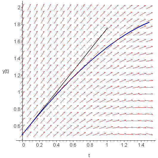
Figure 1 shows Euler's approximation of y(1), that is, following the slope K₀ = f(t₀, y₀) = 1.25, we get that y(t₁) ≈ 0.5 + 1 ⋅ 1.25 = 1.75.

Figure 1. Euler's approximation to the value of y(1).

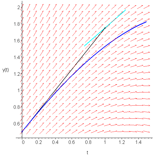
If we sample the slope at (1, 1.75), we find that it is K₁ = f(t₁, y₁) = f(1, 1.75) = 0.875. This slope is shown in Figure 2.

Figure 2. The slope at the point (1, 1.75).

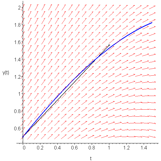
The average of these two slopes is ½(K₀ + K₁) = 1.0625. Therefore, we approximate y(t₁) by following this average slope out a distance 1: y₁ = y₀ + ½(K₀ + K₁)h = 0.5 + 1.0625 ⋅ 1 = 1.5625. This is shown in Figure 3. Note the significant improvement in the approximation as compared to that shown in Figure 1.

Figure 3. Heun's approximation to y(1).

HOWTO

Problem

Given the IVP

y⁽¹⁾(t) = f( t, y(t) )
y(t₀) = y₀

approximate y(t₁).

Assumptions

The function f(t, y) should be continuous in both variables.

Tools

We will use Taylor series.

Initial Conditions

Set h = t₁ − t₀. Let y₁ be the approximation of y(t₁).

Process

Define

K₀ = f( t₀, y₀ ) and
K₁ = f( t₀ + h, y₀ + h K₀ )

Then let

Note that for K₁, t₀ + h = t₁, however we use the above notation to provide similarity with the next topic.

Examples

Example 1

Given the IVP y⁽¹⁾(t) = 1 - t y(t) with y(0) = 1, approximate y(1) with one step.

First, let t₀ = 0, y₀ = 1, and h = 1. Thus, we calculate

K₀ = f(0, 1) = 1
K₁ = f(1, 2) = -1
½(K₀ + K₁) = 0

Therefore, approximation is y₁ = y₀ + h = 1 + 1⋅0 = 1. The actual value is 1.331309118 and therefore the absolute error is approximately 0.331, or approximately half that of what we found using Euler's method.

Example 2

Given the same IVP shown in Example 1, approximate y(0.5).

K₀ = f(0, 1) = 1
K₁ = f(0.5, 1.5) = 0.25
½(K₀ + K₁) = 0.625

Therefore, approximation is y₁ = y₀ + h = 1 + 0.5⋅0.625 = 1.3125. The actual value is 1.342841185 and therefore the absolute error is approximately 0.0303, or approximately 1/8 the error when we used h = 1.

Example 3

Repeat Examples 1 and 2 but with with the initial value y(0.5) = 2.5 and approximating y(1.5) and y(1.0).

First, let t₀ = 0.5, y₀ = 2.5, and h = 1. Therefore

K₀ = f(0.5, 2.5) = -0.25
K₁ = f(1.5, 2.5 - 1 ⋅ 0.25) = -2.375
½(K₀ + K₁) = -1.3125

Therefore, our approximation is y₁ = y₀ + h(-1.3125) = 2.5 + 1(-1.3125) = 1.1875. The actual value is 1.502483616 and therefore the absolute error is approximately 0.315.

Next, let t₀ = 0.5, y₀ = 2.5, and h = 0.5. Therefore

K₀ = f(0.5, 2.5) = -0.25
K₁ = f(1.5, 2.5 - 1 ⋅ 0.25) = -1.375
½(K₀ + K₁) = -0.8125

Therefore, our approximation is y₁ = y₀ + h(-0.8125) = 2.5 + 0.5 (-0.8125) = 2.09375. The actual value is 2.126611964 and therefore the absolute error is approximately 0.0329. Again, the error is approximately 1/8th that of the previous calculation where h = 1.

If we tabulate the errors for various values of h, as is shown in Table 1, we note that as h gets smaller, the error drops by almost exactly 1/8 each time we divide h by two.

Table 1. Errors when approximating y(t₀ + h) for decreasing values of h.

h	Approximation of y(0.5 + h)	Error
1	1.1875	0.315
0.5	2.09375	0.0329
0.25	2.365234375	0.00338
0.125	2.450439453125	0.000366
0.0626	2.479766846	0.0000421
0.03125	2.491031647	0.00000502
0.01625	2.495804310	0.000000612
0.0078125	2.497974455	0.0000000755
0.00390625	2.499005325	0.00000000937

You will note that with each step, the error goes down by approximately a factor of 1/8.

Engineering

To be completed.

Error

To determine the error for Heun's method, we must look at the Taylor series:

Consider the IVP:

y⁽¹⁾(t) = f(t, y(t))
y(t₀) = y₀

We would like to approximate y(t₀ + h). The Taylor series gives us that:

Note that we may approximate the 2nd derivative by taking the forward-divided difference formula [i.e., f⁽¹⁾(x) = (f(x + h) − f(x))/h − ½f⁽²⁾(ξ)h] for the derivative of the 1st derivative:

First, let us denote K₀ = y⁽¹⁾(t₀) = f(t₀, y₀) and note that y(t₀ + h) ≈ y₀ + hK₀.

We also observe that y⁽¹⁾(t₀ + h) = f(t₀ + h, y(t₀ + h)), however, by substituting in our approximation, we have y⁽¹⁾(t₀ + h) ≈ f(t₀ + h, y₀ + hK₀)).

By letting K₁ = f(t₀ + h, y₀ + hK₀)), we may rewrite the approximation as

Substituting these into our Taylor series, we get that:

and by canceling terms, we get:

Therefore, the error is O(h³).

Questions

Question 1

Given the IVP

y⁽¹⁾(t) = 1 - 0.25 y(t) + 0.2 t
y(0) = 1

approximate y(0.5), y(1), and y(1.5) using Heun's method.

Answer: 1.3765625, 1.75625, 2.1390625.

Question 2

Given the same ODE as in Question 1, but with the initial condition y(1) = 2, approximate y(1.5) and y(2.0).

Answer: 2.353125 and 2.7125

Question 3

Given an IVP with an initial condition y(0) = y₀, if the second derivative is bounded by -8 < y⁽³⁾(t) < 8, on how large an interval can we estimate y(t) if we want to ensure that the error is less than 0.0001? Compare this with the range for Question 3 of Euler's method.

Answer: (-0.0531, 0.0531).

Question 4

Consider the following modification to Huen's method:

Instead of defining K₁ = f(t₁, y₀ + hK₀), use this as an initial value and iterate:

K₁ = f(t₁, y₀ + ½h(K₀ + K₁)).

For Question 1, use this modification, iterating the previous step 10 times.

Matlab