Euler's method only samples the slope at the left end-point, that is, the initial point (t0, y0). Let's call this first slope K0 = f(t0, y0). Then if h = t1 - t0, then y1 = y0 + h K0 is Euler's approximation of y(t1).
Let's now sample the slope at this new point (t1, y1), that is, K1 = f(t1, y1). This is only an approximation of the actual slope at y(t1) because y1 is only an approximation of y(t1). Thus, K1 is not as accurate as K0, but let us assume it is still a reasonable approximation.
Therefore, if the change in slope is approximately linear on the interval [t0, t1], then why not use ½(K0 + K1) as a reasonable average value of the slope on the interval?
Thus, use Euler's method to approximate y1 and then use this approximation to approximate K1. Average these two slopes and use this to approximate y1:
Graphical Representation
To view this graphically, let's consider the IVP
y(0) = 0.5
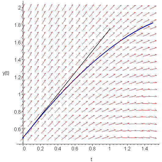
Figure 1 shows Euler's approximation of y(1), that is, following the slope K0 = f(t0, y0) = 1.25, we get that y(t1) ≈ 0.5 + 1 ⋅ 1.25 = 1.75.

Figure 1. Euler's approximation to the value of y(1).
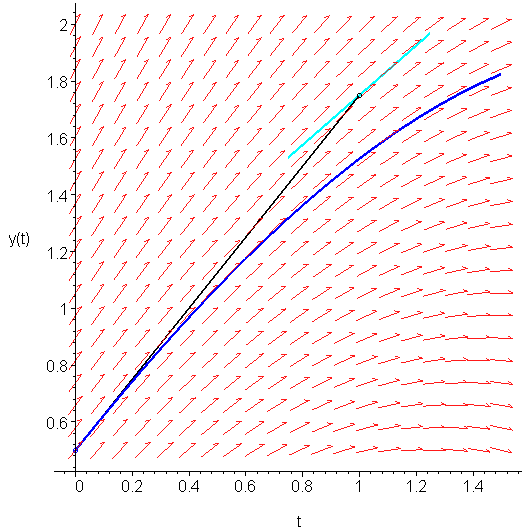
If we sample the slope at (1, 1.75), we find that it is K1 = f(t1, y1) = f(1, 1.75) = 0.875. This slope is shown in Figure 2.

Figure 2. The slope at the point (1, 1.75).
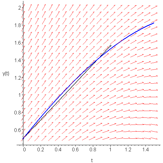
The average of these two slopes is ½(K0 + K1) = 1.0625. Therefore, we approximate y(t1) by following this average slope out a distance 1: y1 = y0 + ½(K0 + K1)h = 0.5 + 1.0625 ⋅ 1 = 1.5625. This is shown in Figure 3. Note the significant improvement in the approximation as compared to that shown in Figure 1.

Figure 3. Heun's approximation to y(1).
Copyright ©2005 by Douglas Wilhelm Harder. All rights reserved.


