Introduction Notes Theory HOWTO Examples Engineering Error Questions Matlab Maple

Example 1

Suppose we are solving Laplace's equation on [0, 1] × [0, 1] with the boundary condition defined by

using h = 0.25.

Ordering the interior points by (1, 1), (1, 2), (1, 3), (2, 1), (2, 2), (2, 3), (3, 1), (3, 2), (3, 3), we associate the following points. Thus, we can associate each of the columns and rows of the matrix as is shown in the matrix<

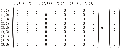
If we evaluate Laplace's equation at the first point, (1, 1), we get:

u_{2, 1} + u_{0, 1} + u_{1, 2} + u_{1, 0} − 4 u_{1, 1} = 0

Two of these points are on the boundary, so we can evaluate the boundary function ∂u at these to get ∂u(0.25, 0) = ∂u(0, 0.25) = 0, and thus, our linear equation simplifies to:

u_{2, 1} + u_{1, 2} − 4 u_{1, 1} = 0

Thus, we fill in the first row of the matirx.

Choosing another point, (3, 2), we get:

u_{4, 2} + u_{2, 2} + u_{3, 3} + u_{3, 1} − 4 u_{3, 2} = 0

This has only one neighbouring boundary-value point where ∂u(1, 0.5) = 1, and therefore, the equation simplifies to:

u_{2, 2} + u_{3, 3} + u_{3, 1} − 4 u_{3, 2} = -1

This defines the 8th row of the matrix, which, if we continue to fill it in, we would get:

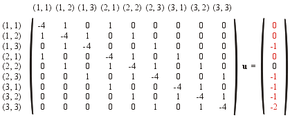
The red entries in the column vector indicate those entries which may have been effected by ∂u on the boundary.

Solving this system of equations yields the vector u = (1/7, 2/7, 1/2, 2/7, 1/2, 5/7, 1/2, 5/7, 6/7)^T. If we plot these points, we get:

Figure 1. The approximation of the solution to Laplace's equation shown in Example 1 with h = 0.25.

If we try this again with h = 0.05, we get the approximations shown in Figure 2.

Figure 2. The approximation of the solution to Laplace's equation shown in Example 1 with h = 0.05.

If we wanted a better approximation, we could use a smaller value of h.

Figure 3. The approximation of the solution to Laplace's equation shown in Example 1 with h = 0.01.

Example 2

Explore what happens when we solve Poisson's equation

for the same boundary conditions as given in Example 1 for values of g between 0 and 4.

u_xx + u_yy = g

Using n = m = 32, Figure 4 shows the approximations for values of g starting with Laplace's equation and going to g = 4.

Figure 4. The solutions to the Poisson equation for values of g ∈ [0, 4].

What Poisson's equation is dictating is that locally, the solution will look like x² + y².

Example 3

Let the boundary condition in Example 1 be replaced by the function cos(π(x + y)). Solve Laplace's equation with this boundary condition.

Using the same ordering of the interior points and using the approximation cos(π/4) ≈ 0.7071, we get the system of linear equations

Solving this system of linear equations, we get the vector

u = 0.35355339, 0, -0.35355339, 0, 0, 0, -0.35355339, 0, 0.35355339)^T

Plotting these points yields the image in Figure 5.

Figure 5. Solving Laplace's equation with sinusoidal boundary conditions.

Using a larger number of points (h = 0.01), we get the approximation shown in Figure 6. Note that the solution looks a lot like the bubble which would result if the wire frame (the boundary) was dipped into soap water.

Figure 6. Solving Laplace's equation with sinusoidal boundary conditions with h = 0.01.

Topic 15.2: Elliptic Partial-Differential Equations (Examples)

Example 1

Example 2

Example 3