

Recall that ux(x, y) is a convenient short-hand notation to represent the first partial derivative of u(x, y) with respect to x. Given the general linear 2nd-order partial-differential equation in two variables:
d(x, y) ux(x, y) + e(x, y) uy(x, y) +
f(x, y) u(x, y) = g(x, y)
Such a PDE is termed elliptical if a(x, y) c(x, y) − b(x, y)2. In the case of constant coefficients, this simplifies to ac − b2. As with the finite-difference method, we can replace each of the partial derivatives with their centred divided-difference formulae, however, we will focus on two forms of this equation, namely, Poisson's equation:
and the special case when g = 0, Laplace's equation:
We will solve Laplace's equation over a connected region R given the value of u(x, y) on the boundary ∂R. Such conditions are referred to as Dirichlet boundary conditions. We will denote such a boundary-value function by ∂u(x, y).
For simplicity, we will start by considering a rectangular region R = [xa, xb] × [ya, yb], as is shown in Figure 1 with the boundary marked in red.
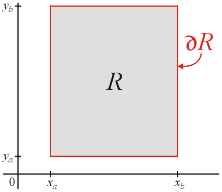
Figure 1. The square region R = [xa, xb] × [ya, yb].
We will assume that xb − xa = nh and yb − ya = mh for appropriate integers n and m, and therefore, we can divide the intervals [xa, xb] and [ya, yb] into n and m sub-intervals, respectively, by defining:
yi = ya + jh
for i = 0, 1, 2, ..., n and j = 0, 1, 2, ..., m. We will try to approximate the value of u(x, y) at each of the points (xi, yi), and thus, we represent these approximation by ui, j ≈ u(xi, yi).
These points and the corresponding approximate values are given in Figure 2. The boundary values are once again marked in red.
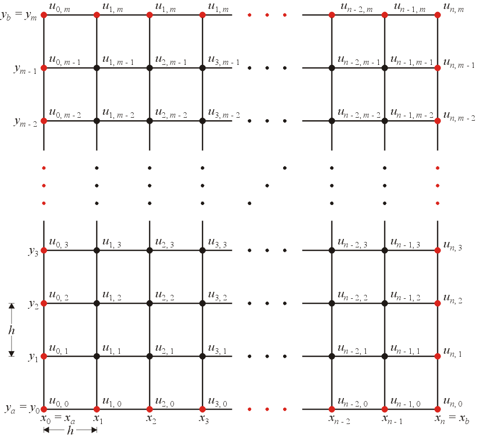
Figure 2. The subdivided region. Click to enlarge.
This region has four boundaries, and from the Dirichlet conditions, we have
ui, m = ∂u(xi, yb)
u0, j = ∂u(xa, yj)
un, j = ∂u(xb, yj)
Therefore, the values at each of the boundary points (red) shown in Figure 2 are known.
The Finite-Difference Equation
The next step is to convert the partial-differential equation into a finite-difference equation. From Topic 13, we can replace each second derivative with its centred divided-difference approximation.
Multiplying by h2, we get:
If g = 0 (Laplace's equation), we note that this simplified to
which is independent of scaling.
Developing the System of Equations
Now, for each interior point (xi, yj) where i = 1, ..., n − 1 and j = 1, ..., m − 1, we can write down the finite difference equation corresponding to those points. For example, given i = 1 and j = 1, we have:
In this case, two of the points are on the border (u0, 1 and u1, 0). From our boundary condition, we can find the value at these point:
This is shown graphically in Figure 3, the two border points (in red) were moved to the right-hand side of the equation.
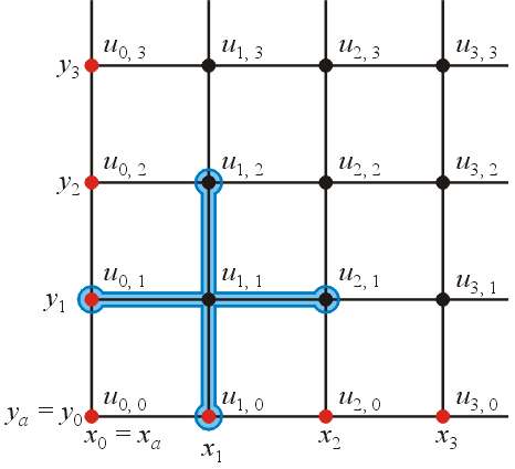
Figure 3. Evaluating the divided-difference formula at (i, j) = (1, 1).
If we repeat this process at i = 2 and j = 1, we have:
In this case, only one of the points is on the border (u2, 0). From our boundary condition, we can find the value at this point:
This is demonstrated in Figure 5.
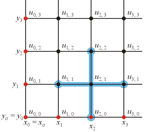
Figure 4. Evaluating the divided-difference formula at (i, j) = (2, 1).
Repeating this process at each interior point, we come up with a system of (n − 1)(m − 1) linear equations in (n − 1)(m − 1) unknowns. Having such a system, we can now solve for the interior values.
Approximating Intermediate Values using Interpolation
We can now use interpolation to estimate intermediate values. For example, suppose that a point (x, y) ∈ [xi − 1, xi] × [xi − 1, xi], then we can find the interpolating bivariate polynomial of the form c1xy + c2x + c3y + c4 by solving
and then evaluating the polynomial at the point (x, y).
Copyright ©2005 by Douglas Wilhelm Harder. All rights reserved.
