The simplex method was introduced by Geogre B. Danzig in 1948 to solve a linear programming problem. For the problem given in the introduction, it involves starting at the origin and then moving along the edges of the polyhedron towards the maximum. It uses linear algebra to follow the edges. Usually it works well, though it can, in very carefully constructed examples, run in exponential time.
Theory
This theory section will begin with an explicit example and then generalize the approach.
Consider the following maximization problem:
Maximize f(x) = 22x1 + 25x2 subject to the constraints:
x1 + x2 ≤ 14
x1 + 2x2 ≤ 22
x1 ≥ 0
x2 ≥ 0
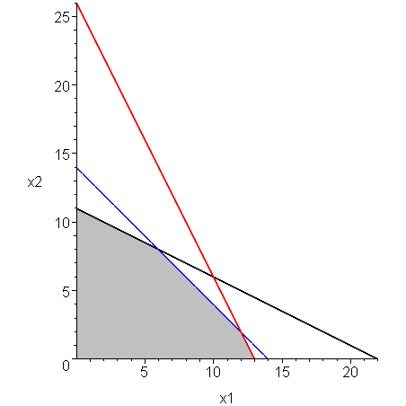
These constraints define the region shown in Figure 1.

Figure 1. The polytope defined by the constraints.
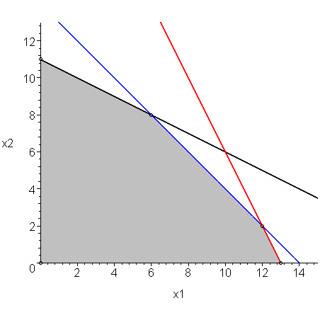
From the theory of linear programming, we know that the maximum of the function f lies at one of the vertexes of the polytope. The vertexes of this polytope (0, 0), (0, 11), (6, 8), (12, 2), (13, 0), shown in Figure 2.

Figure 2. The polytope defined by the constraints.
We could evaluate the function at each of these vertexes, however, this would require us to find all vertexes, a process which could be very expensive. We will now, instead, attempt to derive the method called the simplex method for finding the optimal vertex.
To begin, we can rewrite the set of five inequalities as a system of three linear equations together with a set of five inequalities by introducing three new positive slack variables: x3, x4, x5. We can now write:
x1 + x2 + x4 = 14
x1 + 2x2 + x5 = 22
x1 ≥ 0
x2 ≥ 0
x3 ≥ 0
x4 ≥ 0
x5 ≥ 0
For example, because x3 is required to be positive, if x1 + 2x2 + x3 = 26 is satisfied, then x1 + 2x2 ≤ 26.
The three equations define the matrix
Choosing a Variable
We will start with the solution x = 0 = (0, 0)T. At this point, we note that each step we take in the direction of x1 increases our objective function by 22 while each step in the direction of x2 increases our objection function by 25.
Let us choose x1 to increase first.
Maximizing in the Direction of x1
If we want (x1, 0) to lie on each of the three lines, it follows that:
| Line | Equation | x1 |
|---|---|---|
| 1 | 2x1 + 0 = 26 | 13 |
| 2 | x1 + 0 = 14 | 14 |
| 3 | x1 + 0 = 22 | 22 |
If we use 14, then the first equation is:
∴ x3 = 26 - 28 = -2
This would contradict the requirement that x3 ≥ 0. Therefore, we must assume that our first approximation lies on the first line, and thus we are now at the vertex (13, 0)T. The value of our function at this point is f((13, 0)T) = 22⋅13 + 25⋅0 = 286.
If we evaluate the three equations at this point, we find that the three slack variables are positive:
x4 = 1
x5 = 9
Choosing a Variable
At this point, we note that every increase in the second variable results in an increase of the objective function by 25, but because we are on the line defined by 2x1 + x2, any increase in x2 must result in a corresponding decrease in x1 at half the rate, and therefore a step in the direction of x2 results only in a 25 - 22/2 = 14 net increase in the objective function.
Maximizing in the Direction of x2
To increase the value of x2, we find the intersection between the first line and the next two lines by using Gaussian elimination. To do so, we first begin with the matrix:
To find the intersection of the line defined by the first equation and the next two, we perform Gaussian elimination:
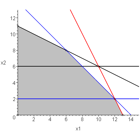
This says that the second line intersects the first when 0.5 x2 = 1 or x2 = 2 and the third line intersects the first when 1.5 x2 = 9 or x2 = 6.
This is shown in Figure 3.

Figure 3. The equations after performing Gaussian elimination.
To chose the next vertex, again, we choose the smaller of the two values. Thus, we use the second line. Solving the first two equations
to get x = (10, 6)T, however, had we substituted this value into the second equation, we would have gotten:
∴x4 = -2
which, again, would contradict the requirement that x4 ≥ 0.
Therefore, we are now at the vertex (12, 2), Δx2 = 2, and therefore f((12, 2)T) = f((13,0)T) + 14 Δx2 = 286 + 28 = 314.
Like before, we have maximized the possible value of x2, and therefore, we will only continue by changing the values of the slack variables x3 and x4. At this point, the value of the function following any line out of x = (12, 2)T is given by the expression 314 + 3x3 - 28x4.
If we evaluate the slack variables at the point (12, 2), we find again that they are all still positive:
x4 = 0
x5 = 6
Choosing a Variable
On this line, we note that each increase in x3 results in a net increase of the objective function by 3 (each increase in x3 results in an increase in x4.
Maximizing in the Direction of x3
At this point, there is only one last line which we can intersect with the line we are current:
Solving this yields x1 = 6 x2 = 8, and x3 = 6. Additionally, if we evaluate the second and third equations at the new point, we find that both slack variables are zero: x4 = x5 = 0, hence all conditions are satisfied.
At this point, we note that:
- Any increase in the second slack variable x4 results in a net decrease in the objective function by 19 (we cannot decrease it because it is already 0), and
- any increase in the slack variable x5 results in a net decrease in the objective by 3 (again, we cannot decrease it because it is already 0).
Because changing any more variables will not increase our objective function, we must be at the optimal vertex, namely, x = (6, 8)T.
The Algorithm
In the howto, we will give an algorithm which solves this problem mechanically.
HOWTO
Problem
Given the linear objective function
subject to a system of system of m linear constraints in n variables, where m ≥ n:
a2,1 x1 + a2,2 x2 + ⋅⋅⋅ a2,n xn ≤ b2
⋅
⋅
⋅
am,1 x1 + am,2 x2 + ⋅⋅⋅ am,n xn ≤ bm
and requiring that each variable is positive
x2 ≥ 0
⋅
⋅
⋅
xn ≥ 0
find a value x which maximizes the function and satisfies the all of the given constraints.
We may write this as maximizing f(x) = cTx subject to Ax ≤ b and x ≥ 0.
Assumptions
The rank of the matrix B is M.
Tools
We will use linear algebra and iteration.
Initial Conditions
Define the matrix
where Idm is the m × m identity matrix and 0m is an m-dimensional column vector. This is an (n + m + 1) × (m + 1) matrix.
Note that the bottom right entry is a simple zero. This is the value of the objective function f at the point x = 0.
The entries of the bottom row (excluding the last entry) are termed indicators. A negative value in this location will indicate that an increase in the variable associated with that column will result in a positive increase in the objective function.
Iterative Process
Select a column j such that the indicator is negative. Select the row i (not including the last) which at the least increases the jth variable (divide the last column by the entry in the jth column choose the smallest positive entry, ignoring any division-by-zeros) to be the pivot.
Perform Gaussian elimination on the jth column using row i as the pivot (add the appropriate multiples of row i to all other rows (including the last row).
For instructive purposes, it is most useful to reduce the matrix to row-reduced echelon form.
Continue doing so until all indicators are positive.
Terminating Conditions
We finish when all indicators are positive. Assuming row-reduced echelon form was used, for each variable x1 through xn for which the column is still in reduced-echelon form read off the value in the last column of the row containing the 1. Otherwise, set the variable to 0.
Examples
Example 1
Maximize f(x) = 22x1 + 25x2 subject to the constraints:
x1 + x2 ≤ 14
x1 + 2x2 ≤ 22
x1 ≥ 0
x2 ≥ 0
We define the matrix
Chose the first column and perform Gaussian elimination and we note of (26/2 = 13, 14/1 = 14 22/1 = 22) that the 1st entry is the smallest positive value, so we perform Gaussian elimination on the 1st column using the 1st row as a pivot to get
Next, we choose the second column and note that of (13/(1/2) = 26, 1/(1/2) = 2, 9/(3/2) = 6), the second is the smallest, and therefore we continue to use Gaussian elimination on the 2nd column using the 2nd row as a pivot.
The third column still has a negative number, and therefore we check that of (12/1 = 12, 2/(−1) = −2, 6/1 = 6), the third has the smallest positive value, and therefore we perform Gaussian elimination based on that variable:
As both variables were visited, we read off from row one that x1 = 6 and from row two x2 = 8. The value of the objective function is 332.
Example 2
Use the same system of constraints as in Example 1, but use the objective function f(x) = x1 + 25x2.
In this case, only the 2nd column is in row-reduced echelon form, and therefore x2 = 11 and x1 = 0. The value of the objective function is 275 (= 11 × 25).
Example 3
Use the same system of constraints as in Example 1, but use the objective function f(x) = 22x1 + x2.
A this point, all indicators are positive, and therefore only one column is reduced, namely, that one corresponding to x1, and therefore our solution is x1 = 13 and x2 = 0, or x = (13, 0)T.
Engineering
To be completed.
Error
As this algorithm is iterative, it does not require error analysis beyond the error analysis associated with the use of double-precision floating-point numbers.
Questions
Question 1
Maximize f(x) = x1 + 2x2 subject to:
x1 + x2 ≤ 2
x1 ≤ 1
x1 ≥ 0
x2 ≥ 0
Answer: x = (1, 1)T.
Question 2
Maximize f(x) = x1 + 2x2 subject to:
x1 + x2 ≤ 4
2x1 + x2 ≤ 6
x1 ≥ 0
x2 ≥ 0
Solution: x = (4/3, 7/3)T.
Question 3
Maximize f(x) = 2x1 + 3x2 + 2x3 subject to:
3x1 + x2 + x3 ≤ 5
x1 + x2 + 2x3 ≤ 4
x1 + x2 + x3 ≤ 3
x1 ≥ 0
x2 ≥ 0
x3 ≥ 0
Answer: x = (1,1,1)T.
Question 4
Maximize f(x) = x1 + 2x2 + x3 subject to:
3x1 + x2 + x3 ≤ 4
x1 + x2 + 2x3 ≤ 4
x1 + x2 + x3 ≤ 2
x1 ≥ 0
x2 ≥ 0
x3 ≥ 0
Solution: x = (0, 0.4, 1.2)T.
Matlab
To be completed later.
Maple
The simplex algorithm is implemented in the simplex package of Maple.
constraints := {3*x + y + z <= 4, 2*x + 2*y + z <= 5, x + 3*y + z <= 4, x + y + 2*z <= 5}; definiteness := {x >= 0, y >= 0, z >= 0}; simplex[maximize]( 3*x + 4*y + 2*z, constraints union definiteness );
        For help on this package or on the maximize routine, enter


?simplex
?simplex,maximize


	Copyright ©2005 by Douglas Wilhelm Harder.  All rights reserved.


