Exponential Distributions
The exponential distribution describes a random variable that follows the distribution
for any value . In this case, the area under the curve is always 1.
The distributions for
are shown in Figure 1.
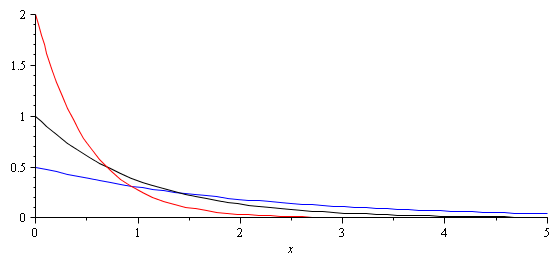
Figure 1. The exponential distributions for (red),
(black), and
(blue).
With any exponential distribution, it is more likely for numbers to be small but positive than it is to be larger. For example, suppose you are expecting about two events to happen per minute (say, a phone call or a request for a web page). If these are independent and an event just happened, how long should you expect to wait until your next event? Because you are expecting two per minute, on average, you would expect to wait thirty seconds, but some times you will wait only 10 seconds and other times you might wait over two minutes. How often should you expect to wait less than 10 seconds and how often should you expect to wait more two minutes?
If such events are independent and there are events per unit time (in this case,
minutes), the arrivals obey an exponential distribution and therefore we can just calculate the
area underneath the curve. To calculate the likelihood that we will wait less than 10 seconds (one sixth of a minute), we calculate
.
Similarly, to determine the probability that you will wait longer than two minutes, we calculate
.
Consequently, you would expect to wait less than 10 seconds approximately 28 % of the time but you would expect to wait over two minutes less than 2 % of the time.
Just to confirm our suspicions, the number of times we should have to wait between 10 seconds and two minutes should therefore be approximately 70 % of the time:
which is what we would expect.
Approximating an Exponential Distribution
Suppose we want to approximate an exponential distribution. In this case, we have a relatively easy way to do this:
The distribution function described above allows you to calculate, for example, the
probability that an event will occur from
to
by calculating
.
Because the area under the curve is 1, we have a 100 % probability that an event will occur at some point.
Next, we ask: what is the probability of an event occurring before time ? In this case,
we must calculate
.
We define the cumulative distribution function to be
.
In the case of the exponential distribution, we get
.
The cumulative distribution functions for are shown in Figure 2.
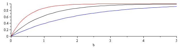
Figure 1. The exponential cumulative distributions for (red),
(black), and
(blue).
Now, the cumulative distribution function must have some properties:
- In the limit, as
,
,
- In the limit, as
,
, and
- The function must be monotonic increasing: if
, then
.
We can use this to approximate an exponential distribution by choosing a random number on and calculating
the inverse of the cumulative distribution function. Suppose
is a random number between
and
: then
will give a value that matches the distribution. In this case, the inverse
is
.
Notice that because , then
, and thus
and
therefore
because
.
Note: the natural logarithm, is normally implemented as the log(x) function in most mathematical packages.
The following C program, stored in exponential.c in the source directory, generates and prints 100 events with a given value of LAMBDA:
#include <stdlib.h>
#include <stdio.h>
#include <math.h>
#include <time.h>

#define LAMBDA 0.7
#define N      100

int main() {
	double event[N];
	int i;

	srand48( time( NULL ) );

	event[0] = 0.0;

	for ( i = 1; i < N; ++i ) {
		double x;

		x = drand48();
		event[i] = event[i - 1] - log( 1 - x )/LAMBDA;
	}

	printf( "%f", event[0] );

	for ( i = 1; i < N; ++i ) {
		printf( ", %f", event[i] );
	}

	printf( "\n" );

	return 0;
}
When compiled and executed, one version of the output is
% gcc -lm exponential.c
% ./a.out
0.000000, 0.458627, 0.747179, 3.792151, 4.622758, 6.811202, 7.085109, 9.490516, 10.664299,
13.211029, 14.657234, 15.381296, 15.423190, 16.213358, 21.695082, 21.991026, 23.119533,
27.029755, 29.357154, 30.766622, 31.337770, 33.316074, 33.705675, 37.254324, 37.304430,
39.341405, 40.356964, 41.627228, 42.826582, 45.365113, 46.759513, 47.570298, 48.077224,
49.115887, 51.513948, 54.626003, 55.453093, 56.604780, 58.149573, 58.671860, 58.778942,
60.157318, 60.557956, 65.566854, 65.952261, 67.282563, 69.689630, 70.597455, 71.018470,
71.333150, 72.010313, 72.637144, 73.353536, 76.406307, 77.691911, 80.091032, 81.415478,
81.500078, 83.437088, 84.698901, 85.424763, 86.488556, 87.318447, 88.599910, 89.453325,
89.730148, 91.743414, 92.401052, 94.159618, 98.376016, 99.069261, 105.508869, 106.104842,
106.578099, 107.299884, 108.663510, 109.970127, 110.221565, 111.134777, 111.357513,
112.092976, 115.063179, 116.530103, 116.705686, 118.008703, 119.570930, 122.027815,
122.281497, 122.425214, 122.928374, 123.352518, 123.606629, 124.554290, 129.030988,
130.804370, 134.348100, 134.401448, 134.554584, 135.280998, 137.177269
With events per unit time, we would expect 100 events to
occur in
units of time which is reasonably
close to what we found. If you execute the program a number of times, you will see that some
times the 100 events occur in less than 143 units and at other times it will be greater than;
however, if you were to run the program many times, on average, it will be very close to
143 units of time.
Other Applications of the Exponential Distribution
The exponential distribution can be used for measuring distance between random events, including mutations on a strand of DNA. It can also be used for the time interval between radioactive decays allowing estimating of half lives on the order of millions or billions of years. It is also very useful in reliability engineering where it can be used to model a constant hazard rate.
Estimating the Parameter λ
If you have a real-world situation which you believe can be modeled by an exponential distribution,
you can estimate by taking the inverse of the average the time intervals between events or
dividing the number of events that occurred in a period of time by the the length of that period.
For example, suppose the following events occurred:
0.927, 0.951, 0.989, 1.136, 1.570, 1.950, 2.962, 3.102, 3.921
in a period of four seconds. In that case,
would estimate the time. Similarly, taking the average of the times between the events
gives
, the inverse of which is
.
Note that this only estimates the value of : the actual
value may be slightly different (although, the more samples you take, the closer your
estimation will be).

Department of Electrical and Computer Engineering
University of Waterloo
200 University Avenue West
Waterloo, Ontario, Canada N2L 3G1
Website maintained by Douglas Wilhelm Harder