Normal Distributions
Approximating a Standard Normal Distribution
The following algorithms approximate a normal distribution: that is, a normal distribution
with a mean of and a standard deviation of
. To approximate
a normal distribution with mean
and a standard deviation
,
generate a random variable
from a standard normal distribution and then
calculate
.
Four algorithms are implemented, including:
- Approximating the normal distribution with twelve uniform deviates,
- The Box-Muller method,
- The ratio method, and
- The Marsaglia polar method.
The adds twelve uniform deviates from [0, 1] and subtracts six. By the central limit theorem, this has a mean of 0 and a standard deviation of 1.
The Box-Muller method samples from a bivariate normal distribution and produces normal deviates in pairs. The implementation alternates between calculating two normal deviates, storing one; and returning the stored deviate.
The ratio method is explained in the referenced text by Knuth but requires the calculation of only one natural logarithm.
The Marsaglia polar method is an alternate formulation of the Box-Muller method that does not require the computation of the two trigonometric functions.
Of the four algorithms, Table 1 demonstrates that the Marsaglia polar method is the fastest, but summing twelve uniform deviates is slower only by a factor of two.
Table 1. Timings for the four algorithms.
| Algorithm | Relative Time | Function Calls |
|---|---|---|
| Marsaglia polar method | 1.000 | sqrt,log |
| Box-Muller method | 1.488 | sqrt,log,sin,cos |
| Ratio method | 1.756 | log |
| Central Limit Theorem | 2.183 | none |
While the ratio method does not require the evaluation of as many functions, the there is a step that has a much higher probability of looping.
The 12-Sample Approximation
While the Box-Muller, ratio and Marsaglia polar methods all produce points that follow the distribution, but the first method produces only an approximation. The distribution of the sum of the twelve distributions is given the piecewise polynomial function
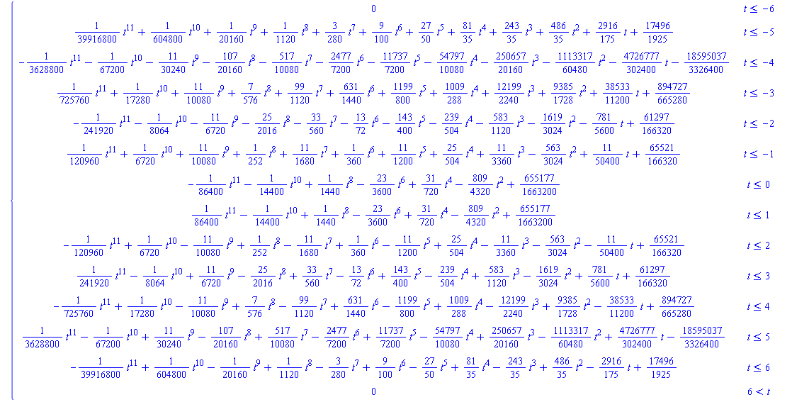 .
.
The integral of this rather complex function is 1 and it is reasonably close to a normal
distribution, as is shown in Figure 2 which plots both this approximation and the standard
normal distribution and Figure 3
which plots the difference between the two functions. On the interval [-2.5, 2.5], the
relative error is less than 2.5%; thus, this is for many basic applications a very
reasonable approximation of a standard normal distribution.
Figure 2. A plot of the approximation (red) and the standard normal distribution (blue).
Figure 3. A plot of the difference between the approximation and the standard normal distribution.

Department of Electrical and Computer Engineering
University of Waterloo
200 University Avenue West
Waterloo, Ontario, Canada N2L 3G1
Website maintained by Douglas Wilhelm Harder