Laboratory 1

Slides for this presentation are available here: 1.BVPs.pptx. The presentation for this talk is available on youtube.

The laboratory may be downloaded from UW Learn and is to be submitted there. Be sure to add your name or names, any UW User IDs, and any other information in the file name and on the Laboratory title page.

Conventions

To differentiate between time and space, we will use $x$, ${\bf x} = (x, y)^T$, and ${\bf x} = (x, y, z)^T$ to represent 1, 2, and 3 dimensional spaces and the approximation of the functions at various points by $u(x_{i_x}) \approx u_k$, $u(x_{i_x}, y_{i_y}) \approx u_{j,k}$, and $u(x_{i_x}, y_{i_y}, z_{i_z}) \approx u_{i_x, i_y, i_z}$. The change in variable is there to ensure clarity: it is more likely to mistake i and j and 1 as opposed to k.

The time variable will be indexed by the letter $k$: $t_k$ and we will approximate solutions $u(t_k) \approx u_t$, $u(x_{i_x}, t_k) \approx u_{i_x, k}$, $u(x_{i_x}, y_{i_y}, t_k) \approx u_{i_x, i_y, k}$, and $u(x_{i_x}, y_{i_y}, z_{i_z}, t_k) \approx u_{i_x, i_y, i_z, k}$.

Introduction

Solutions to partial-differential equations of interest to electrical and computer engineers usually include one or more space dimension (labeled x, y, and z; though we may write the space dimension as a vector x) and usually a time dimension (labeled t). The solution will be denoted as u(x, t).

Boundary-value Problems

In general, the conditions on the space dimension define the system on the boundary: in one dimension, this says that we define the system at two points a and b and that the solution between those two points is defined by $u(a, t)$ and $u(b, t)$.

The simplest example is that where a system contains only one space dimension and does not depend on time, in which case the boundary-value problem is reduced to defining $u(a) = u_a$ and $u(b) = u_b$.

In general, a second-order ordinary differential equation is of the form

$f(x, u, u^{(1)}, u^{(2)}) = 0$

where the solution is a function $u(x)$ and this defines a boundary-value problem when the system is constrained to satisfy $u(a) = u_a$ and $u(b) = u_b$.

We will, however, not consider the general case and instead focus on numerical solutions the linear case of the form

$c_1 u^{(2)}(x) + c_2 u^{(1)}(x) + c_3 u(x) = g(x)$.

(1)

To solve such a problem numerically requires approximations of the the first and second derivatives. From MATH 211, we know that

$u^{(1)}(x) \approx \frac{u(x + h) - u(x - h)}{2h} + O(h^2)$

and

$u^{(2)}(x) \approx \frac{u(x + h) - 2u(x) + u(x - h)}{h^2} + O(h^2)$.

Substituting these into Equation 1 yields

$c_1 \frac{u(x + h) - 2u(x) + u(x - h)}{h^2}+ c_2 \frac{u(x + h) - u(x - h)}{2h} + c_3 u(x) = g(x)$.

Multiplying this equation by $2h^2$ to eliminate any denominator yields

$2 c_1 \left(u(x + h) - 2u(x) + u(x - h)\right ) + h c_2 \left( u(x + h) - u(x - h) \right) + 2h^2 c_3 u(x) = 2h^2 g(x)$

which can be expanded and collected on the terms $u(x - h)$, $u(x)$ and $u(x + h)$:

$\left( 2 c_1 - hc_2 \right ) u(x - h) + \left( 2h^2c_3 - 4c_1 \right ) u(x) + \left( 2c_1 + hc_2 \right ) u(x + h) = 2h^2 g(x)$.

(2)

Equation 2 gives us a discrete version approximation of the linear 2nd-order ordinary differential equation shown in Equation (1). Consequently, a solution which satisfies Equation 2 should be an approximate solution of Equation 1.

To make use of this equation, we will first simplify the appearance by defining three new functions:

$d^- = 2 c_1 - hc_2$,
$d = 2h^2c_3 - 4c_1$, and
$d^+ = 2 c_1 + hc_2$.

We can therefore rewrite Equation 2 as

$d^- u(x - h) + d u(x) + d^+ u(x + h) = 2h^2 g(x)$.

(3)

To make use of this, we first realize that given the boundary values $(a, u_a)$ and $(b, u_b)$; we need to approximate the solution on the interval $[a, b]$ and therefore, the logical approach would be to divide the interval into $n$ sub-intervals of width $h = \frac{b - a}{n - 1}$ where $x_{i_x} = a + (k - 1)h$ and therefore $x_1 = a$ and $x_n = b$. These points are shown in Figure 1.

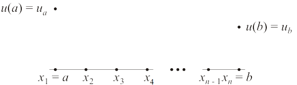
Figure 1. Dividing the interval $[a, b]$ into n points.

We would like to find approximate values of the solution for each of the interior points $u(x_2), u(x_3), \ldots, u(x_{n - 1})$ and therefore, we will denote these unknown approximate values by $u(x_{i_x}) \approx u_k$ for $k = 2, 3, \ldots, n - 1$ and and for completeness, we note that the values are defined at the end points: $u(x_1) = u_a = u_1$ and $u(x_n) = u_b = u_n$. This is demonstrated in Figure 2.

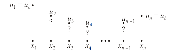
Figure 2. Denoting the unknown values.

For each of the interior points, we can substitute these into Equation 3 and we note that if $u(x_{i_x}) \approx u_k$, it follows that, by our definitions, $u(x_{i_x} - h) \approx u_{k - 1}$ and $u(x_{i_x} + h) \approx u_{k + 1}$. Therefore we have

Substituting $x = x_1$:

$d^- u_1 + d u_2 + d^+ u_3 = 2h^2 g(x_2)$,

substituting $x = x_2$:

$d^- u_2 + d u_3 + d^+ u_4 = 2h^2 g(x_3)$,

substituting $x = x_3$:

$d^- u_3 + d u_4 + d^+ u_5 = 2h^2 g(x_4)$,

..., substituting $x = x_{n - 2}$:

$d^- u_{n - 3} + d u_{n - 2} + d^+ u_{n - 1} = 2h^2 g(x_{n - 2})$, and

substituting $x = x_{n - 1}$:

$d^- u_{n - 2} + d u_{n - 1} + d^+ u_n = 2h^2 g(x_{n - 1})$.

Recalling, however, the two boundary values, this allows us to rewrite these equations as

$d u_2 + d^+ u_3 = 2h^2 g(x_2) - d^- u_a$,
$d^- u_2 + d u_3 + d^+ u_4 = 2h^2 g(x_3)$,
$d^- u_3 + d u_4 + d^+ u_5 = 2h^2 g(x_4)$,
$\vdots$
$d^- u_{n - 3} + d u_{n - 2} + d^+ u_{n - 1} = 2h^2 g(x_{n - 2})$
$d^- u_{n - 2} + d u_{n - 1} = 2h^2 g(x_{n - 1}) - d^+ u_b$.

A cursory glance shows that this is a linear system of $n - 2$ in the $n - 2$ unknowns $u_2, u_3, u_4, ..., u_{n - 2}, u_{n - 1}$; therefore, we may use linear algebra to solve the problem

$\begin{pmatrix} d & d^+ & & & & \cr d^- & d & d^+ & & & \cr & d^- & d & d^+ & & \cr & & \ddots & \ddots & \ddots & \cr & & & d^- & d & d^+ \cr & & & & d^- & d \end{pmatrix} \begin{pmatrix} u_2 \cr u_3 \cr u_4 \cr \vdots \cr u_{n - 2} \cr u_{n - 1} \end{pmatrix}= \begin{pmatrix} 2h^2 g(x_2) - d^-u_a \cr 2h^2 g(x_3) \cr 2h^2 g(x_4) \cr \vdots \cr 2h^2 g(x_{n - 2}) \cr 2h^2 g(x_{n - 1}) - d^+u_b \end{pmatrix}$.

Homogeneous Equations

If the differential equation is homogeneous, that is, $g(x) = 0$, it follows that the system may be further simplified to

$\begin{pmatrix} d & d^+ & & & & \cr d^- & d & d^+ & & & \cr & d^- & d & d^+ & & \cr & & \ddots & \ddots & \ddots & \cr & & & d^- & d & d^+ \cr & & & & d^- & d \end{pmatrix} \begin{pmatrix} u_2 \cr u_3 \cr u_4 \cr \vdots \cr u_{n - 2} \cr u_{n - 1} \end{pmatrix} = \begin{pmatrix} -d^-u_a \cr 0 \cr 0 \cr \vdots \cr 0 \cr -d^+ u_b \end{pmatrix}$.

In this last case, you will note that the solution is independent of h and is therefore scale independent.

Examples of Numerical Solutions to Boundary-value Problems

We will look at six boundary-value problems, five of which have solutions and one for which an exact solution does not exists. The last example, in a sense, the most trivial, will oddly enough, be referred to in many future examples with the heat conduction/diffusion equation and the wave equation.

In each of the examples, the boundary conditions will be $u(0) = 0$ and $u\left(\frac{\pi}{2}\right) = 1$—only the linear ordinary differential equation will change. In each case, we will use approximate the solution on 7 interior points.

Example 1

The solution to the differential equation

$u^{(2)}(x) + u(x) = 0$

(4)

is shown in Figure 3.

Figure 3. The solution to the ODE in Equation 4 with boundary values $u(0) = 0$ and $u\left(\frac{\pi}{2}\right) = 1$.

By inspection, the solution is $u(x)= \sin(x)$.

With $n = 9$, the resulting 7 × 7 matrix is

M =

  -3.92289   2.00000   0.00000   0.00000   0.00000   0.00000   0.00000
   2.00000  -3.92289   2.00000   0.00000   0.00000   0.00000   0.00000
   0.00000   2.00000  -3.92289   2.00000   0.00000   0.00000   0.00000
   0.00000   0.00000   2.00000  -3.92289   2.00000   0.00000   0.00000
   0.00000   0.00000   0.00000   2.00000  -3.92289   2.00000   0.00000
   0.00000   0.00000   0.00000   0.00000   2.00000  -3.92289   2.00000
   0.00000   0.00000   0.00000   0.00000   0.00000   2.00000  -3.92289

b =
   0
   0
   0
   0
   0
   0
   2

and

u = [0; M \ b; 1]

u =

   0.00000
   0.19540
   0.38327
   0.55636
   0.70800
   0.83235
   0.92461
   0.98122
   1.00000

plot( linspace( 0, pi/2, 9 ), u, 'o' );

The approximations are shown in Figure 4.

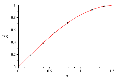
Figure 4. The seven approximations to the solution in Figure 3.

Example 2

The solution to the differential equation

$u^{(2)}(x) + 2u(x) + u(x) = 1$

(5)

is shown in Figure 5.

Figure 5. The solution to the ODE in Equation 5 with boundary values $u(0) = 0$ and $u\left(\frac{\pi}{2}\right) = 1$.

The solution to this boundary-value problem is $u(x)= 1 - e^{-x} + \frac{2}{\pi}xe^{-x}$.

The approximations when using $n = 9$ are shown in Figure 6.

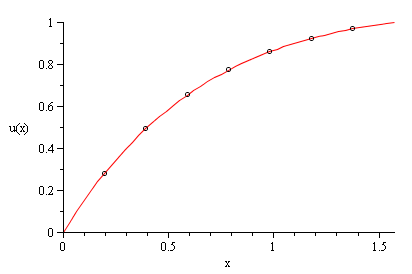
Figure 6. The seven approximations to the solution in Figure 5.

Example 3

The solution to the differential equation

$u^{(2)}(x) - 5u'(x) + 3u(x)= 7$

(6)

is shown in Figure 7.

Figure 7. The solution to the ODE in Equation 6 with boundary values $u(0) = 0$ and $u\left(\frac{\pi}{2}\right) = 1$.

The approximations are shown in Figure 8.

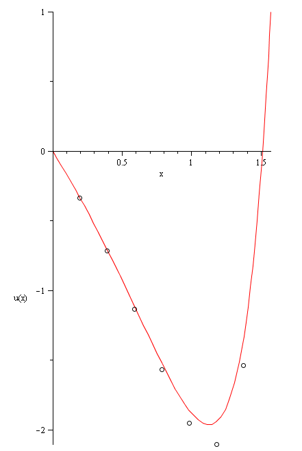
Figure 8. The seven approximations to the solution in Figure 7.

This is also an excellent opportunity to demonstrate that the convergence of the divided difference is O(h²), that is, reducing h by a factor of two reduces the absolute error by a factor of four. Of course, this requires calculating the divided difference at an exponentially increasing number of points.

This code fragment selects the approximation of the solution at $x = \frac{3pi}{8}$ with twice as many points for each subsequent approximation:

v = zeros( 10, 1 );
for i = 1:10
      [xpts, upts] = bvp( [1 -5 3], @g, [0 pi/2], [0 1], 4*2^i + 1 )
      v(i) = upts(end - 2^i);
end

Inspecting these absolute values yields the table

0.158761808926688
0.037392460692664
0.009217227356775
0.002296302879338
0.000573578215540
0.000143363564911
0.000035839009553
0.000089596924060
0.000022400068442
0.000055968541224

You will note that with each step, the error is reduced by approximately by a factor of 4.

NE 217 Advanced Calculus 2 for Nanotechnology Engineering

Laboratory 1

Conventions

Introduction

Boundary-value Problems

Homogeneous Equations

Examples of Numerical Solutions to Boundary-value Problems

Example 1

Example 2

Example 3