Extrapolation is the process of taking data values at points x1, ..., xn, and approximating a value outside the range of the given points. This is most commonly experienced when an incoming signal is sampled periodically and that data is used to approximate the next data point. For example, weather predictions take historic data and extrapolate a future weather pattern. Sensors may take the current and past voltages of an incoming signal and approximate a future value, perhaps attempting to compensate more appropriately.
Background
Useful background for this topic includes:
Theory
We have seen how to use interpolation to approximate values between points x1, ..., xn, and in many cases, the error of the approximations of the points near the center of the x values is quite accurate. However, if we are trying to approximate a value at a value outside the range of x values, the error increases significantly when using interpolation. However, if model information is available, for example, that the data is linear, quadratic, or exponential, we may use least-squares to find a best-fitting curve. It can be shown that the error associated with extrapolating a least-squares fitting curve is significantly less than the error associated with extrapolating an interpolating polynomial.
Thus, for example, if you are given the points
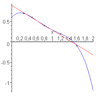
and wish to approximate the value at 2.0, then we can do nothing which may give us a good approximation. If, however, we are told that this data is linear, then we may find the least-squares fitting line (y(x) = -0.60830 x + 0.89531), then we may approximate the value at x = 2 by evaluating this function: y(2) = -0.60830⋅2 + 0.89531 = -0.32130.
The data, the interpolating polynomial (blue), and the least-squares line (red) are shown in Figure 1. The appropriateness of the extrapolating estimator should be apparent.

Figure 1. Extrapolation of exponentially decaying points in Example 4.
If you take nothing else from this topic, remember: you cannot use an interpolating polynomial to extrapolate a value. To successfully extrapolate data, you must have correct model information, and if possible, use the data to find a best-fitting curve of the appropriate form (e.g., linear, exponential) and evaluate the best-fitting curve on that point.
HOWTO
Problem
Given data (xi, yi), for i = 1, 2, ..., n, extrapolate a value outside the range of x values.
Assumptions
We will assume the data is correctly modeled by a curve on which we may either apply linear regression, or may apply a transformation to linear regression.
Tools
We will use linear regression.
Process
Find the least-squares regression curve, and evaluate that function at that point.
The error in our extrapolated value depends on how far we are from the mean of the x values.
Examples
Example 1
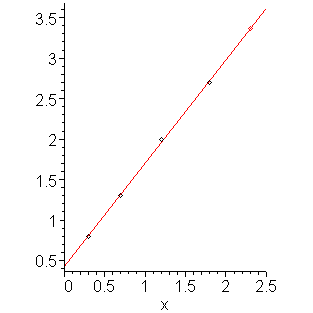
Given the following data which is known to be linear, extrapolate the y value when x = 2.3.
The best fitting line is y(x) = 1.27778 x + 0.42222, and therefore our approximation of the value at 2.3 is 3.3611. The points, the least-squares fitting line, and the extrapolated point are shown in Figure 1.

Figure 1. Extrapolation of points in Example 1.
Example 2
Given the following data which is known to be linear, use Matlab to extrapolate the y value when x = 4.5.
(0.90105, 1.05687), (1.21687, 1.18567), (1.47891, 1.23277),
(1.52135, 1.25152), (3.25427, 1.79252), (3.42342, 1.85110),
(3.84589, 1.98475)
In Matlab:
>> x = [0.01559 0.30748 0.31205 0.90105 1.21687 1.47891 1.52135 3.25427 3.42342 3.84589]';
>> y = [0.73138 0.91397 0.83918 1.05687 1.18567 1.23277 1.25152 1.79252 1.85110 1.98475]';
>> V = [x x.^0];
>> c = V \ y
c =

  0.31722
  0.76764

>> polyval( c, 4.5 )
ans = 2.1951
>> polyval( c, 4.5 )
We can plot the points with the following additional commands:
>> plot( x, y, 'o' );
>> xs = 0:5;
>> ys = polyval( c, xs );
>> hold on
>> plot( xs, ys );
Example 3
Consider the following data:
Using extrapolation with a linear function and a quadratic function to estimate the value of x = 1.5. Comment.
(0.24253, -0.00397), (0.27129, 0.01410), (0.31244, 0.08215),
(0.51378, 0.04926), (0.59861, 0.14643), (0.63754, 0.08751)
Using Matlab:
>> x = [-0.73507 -0.58236 -0.22868 0.24253 0.27129 0.31244 0.51378 0.59861 0.63754]';
>> y = [0.17716 0.13734 0.00741 -0.00397 0.01410 0.08215 0.04926 0.14643 0.08751]';
>> V = [x x.^0];           % Linear
>> c1 = V \ y
c1 =
  -0.0455620
   0.0827014
>> polyval( c1, 1.5 )
ans = 0.014358
>> V = [x.^2 x x.^0];
>> c2 = V \ y
c2 =
   0.30768
  -0.01834
   0.00470
>> polyval( c2, 1.5 )
ans = 0.66947
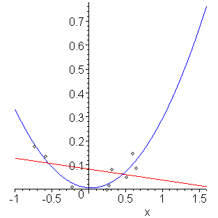
We note that both techniques give answers, but if we plot both the points and the interpolating polynomials, as shown in Figure 2, we note that the quadratic function seems to fit the points better. Additionally, looking at the coefficients, the second polynomial suggests that the actual form of the data may be y(x) = 0.30768 x2.

Figure 2. Extrapolation of points in Example 3.
Example 4
Suppose the following data comes from an exponentially decreasing phenomena, for example, discharge on a capacitor. When will the the charge be half the charge at time t = 0?
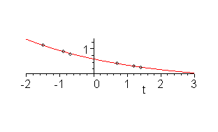
Using the exponential transformation, we get that the best fitting exponential function is y(t) = 0.69830 e-0.30421 t, and therefore, the estimated half-life is t = log(2)/0.30421 = 2.2785. The points and the least-squares exponential function are shown in Figure 3.
The calculation of the half-life is a form of extrapolation.

Figure 3. Extrapolation of exponentially decaying points in Example 4.
Engineering
In engineering, it will always be necessary to extrapolate, given data from the present and previous time, to some point in the future. For example, it is possible to take the current voltages of a system, and it may be necessary, in order to respond appropriately to a system, to extrapolate a future value.
For example, assuming that the input is known (from our model) to have a constant rate of change, it would be more appropriate to take the last four or five sampled points (depending on how much computing power is available) and find a least-squares linear polynomial than it would be to take just the last two points and find the interpolating linear polynomial, especially if it is known that the measurement error may be large.
To demonstrate the extreme case, consider the data where the measurement is severely truncated:
0 0 0 0 1 1 1 1 2 2 2 2 3 3 3 3 4 4 4 4
however, the measurements still to be from a source which is linear.
If we use two points and interpolation to approximate the next value, we get the following:
    0 0 0 0 1 1 1 1 2 2 2 2 3 3 3 3 4 4 4 4
        0 0 0 2 1 1 1 3 2 2 2 4 3 3 3 5 4 4 4
Note how only half of the approximations are reasonable predictors of future behaviour. If now, instead, we use the least squares fit of all previously known points, we have the following predictions (where we use rounding):
    0 0 0 0 1 1 1 1 2 2 2 2 3 3 3 3 4 4 4 4
      0 0 0 0 1 1 1 1 2 2 2 2 3 3 3 4 4 4 4 5
The prediction becomes better with each passing point. Of course, this applies only if we know from the model that the input has a constant rate-of-change.
Because of the severe truncation error, this example benefited most from maintaining all previous data in extrapolating the next point. This would not be difficult to calculate quickly: each entry of VTV and VTy could be easily updated with six additions.
Error
The error associated with extrapolation is beyond the scope of this course, but if it is assumed that the data is normally distributed, it can be shown that the error is quite easy to calculate, and for examples, when the data is known to be linear, then the error of extrapolation only increases quadratically as you move away from the average of the x values and the corresponding coefficient is significantly smaller than that for using an interpolating polynomial with only two points. In fact, it can be shown that any extrapolation using an interpolating linear function has no statistical significance. It is like using a single point to estimate a mean: you cannot say anything about the error associated with your estimator.
To demonstrate this last point, consider finding the average height of all humans by taking just one human. While 5'11" may be an approximation to the mean, no information about how good this estimator is is available. Even if we randomly sample two humans and average their heights, we can find bounds for the actual average which are correct 19 times out of 20 (assuming we have a random sample).
Questions
Question 1
Use extrapolation to approximate the the value of x = 3 for the given data (known to be linear):
Answer: -6.5
Question 2.
Use extrapolation to approximate the value of x = 3 for the given data (known to be of the form y(x) = c1x2.
Answer: y = 39/34 ⋅ 32 ≈ 10.323.
Matlab
Extrapolation in Matlab is done using the techniques used in the previous sub-topics of linear regression, as appropriate.
Maple
Extrapolation in Maple is done using the techniques used in the previous sub-topics of linear regression, as appropriate.
Copyright ©2005 by Douglas Wilhelm Harder. All rights reserved.


