Introduction Notes Theory HOWTO Examples Engineering Error Questions Matlab Maple

Example 1

Given the following data which is known to be linear, extrapolate the y value when x = 2.3.

(0.3 0.80), (0.7, 1.3), (1.2, 2.0), (1.8, 2.7)

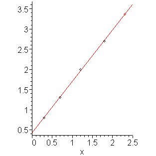
The best fitting line is y(x) = 1.27778 x + 0.42222, and therefore our approximation of the value at 2.3 is 3.3611. The points, the least-squares fitting line, and the extrapolated point are shown in Figure 1.

Figure 1. Extrapolation of points in Example 1.

Example 2

Given the following data which is known to be linear, use Matlab to extrapolate the y value when x = 4.5.

(0.01559, 0.73138), (0.30748, 0.91397), (0.31205, 0.83918),
(0.90105, 1.05687), (1.21687, 1.18567), (1.47891, 1.23277),
(1.52135, 1.25152), (3.25427, 1.79252), (3.42342, 1.85110),
(3.84589, 1.98475)

In Matlab:

>> x = [0.01559 0.30748 0.31205 0.90105 1.21687 1.47891 1.52135 3.25427 3.42342 3.84589]';
>> y = [0.73138 0.91397 0.83918 1.05687 1.18567 1.23277 1.25152 1.79252 1.85110 1.98475]';
>> V = [x x.^0];
>> c = V \ y
c =

  0.31722
  0.76764

>> polyval( c, 4.5 )
ans = 2.1951
>> polyval( c, 4.5 )

We can plot the points with the following additional commands:

>> plot( x, y, 'o' );
>> xs = 0:5;
>> ys = polyval( c, xs );
>> hold on
>> plot( xs, ys );

Example 3

Consider the following data:

Using extrapolation with a linear function and a quadratic function to estimate the value of x = 1.5. Comment.

(-0.73507, 0.17716), (-0.58236, 0.13734), (-0.22868, 0.00741),
(0.24253, -0.00397), (0.27129, 0.01410), (0.31244, 0.08215),
(0.51378, 0.04926), (0.59861, 0.14643), (0.63754, 0.08751)

Using Matlab:

>> x = [-0.73507 -0.58236 -0.22868 0.24253 0.27129 0.31244 0.51378 0.59861 0.63754]';
>> y = [0.17716 0.13734 0.00741 -0.00397 0.01410 0.08215 0.04926 0.14643 0.08751]';
>> V = [x x.^0];           % Linear
>> c1 = V \ y
c1 =
  -0.0455620
   0.0827014
>> polyval( c1, 1.5 )
ans = 0.014358
>> V = [x.^2 x x.^0];
>> c2 = V \ y        
c2 =
   0.30768
  -0.01834
   0.00470
>> polyval( c2, 1.5 )
ans = 0.66947

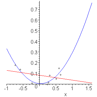
We note that both techniques give answers, but if we plot both the points and the interpolating polynomials, as shown in Figure 2, we note that the quadratic function seems to fit the points better. Additionally, looking at the coefficients, the second polynomial suggests that the actual form of the data may be y(x) = 0.30768 x².

Figure 2. Extrapolation of points in Example 3.

Example 4

Suppose the following data comes from an exponentially decreasing phenomena, for example, discharge on a capacitor. When will the the charge be half the charge at time t = 0?

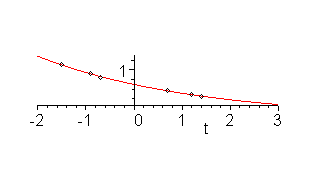
(-1.5, 1.11), (-0.9, 0.92), (-0.7, 0.85), (0.7, 0.57), (1.2, 0.49), (1.4, 0.45)

Using the exponential transformation, we get that the best fitting exponential function is y(t) = 0.69830 e^{-0.30421 t}, and therefore, the estimated half-life is t = log(2)/0.30421 = 2.2785. The points and the least-squares exponential function are shown in Figure 3.

The calculation of the half-life is a form of extrapolation.

Figure 3. Extrapolation of exponentially decaying points in Example 4.

Topic 6.4: Extrapolation (Examples)

Example 1

Example 2

Example 3

Example 4