Introduction Notes Theory HOWTO Examples Engineering Error Questions Matlab Maple

The false-position method is a modification on the bisection method: if it is known that the root lies on [a, b], then it is reasonable that we can approximate the function on the interval by interpolating the points (a, f(a)) and (b, f(b)). In that case, why not use the root of this linear interpolation as our next approximation to the root?

Background

Useful background for this topic includes:

3. Iteration
5. Interpolation

5.1 Vandermonde Method

8. Bracketing

References

Bradie, Section 2.2, The Method of False Position, p.71.
Mathews, Section 2.2, p.56.
Weisstein, http://mathworld.wolfram.com/MethodofFalsePosition.html.

Theory

The bisection method chooses the midpoint as our next approximation. However, consider the function in Figure 1.

Figure 1. A function on an interval [6, 8].

The bisection method would have us use 7 as our next approximation, however, it should be quite apparent that we could easily interpolate the points (6, f(6)) and (8, f(8)), as is shown in Figure 2, and use the root of this linear interpolation as our next end point for the interval.

Figure 2. The interpolating linear polynomial and its root.

This should, and usually does, give better approximations of the root, especially when the approximation of the function by a linear function is a valid. This method is called the false-position method, also known as the reguli-falsi. Later, we look at a case where the the false-position method fails because the function is highly non-linear.

Halting Conditions

The halting conditions for the false-position method are different from the bisection method. If you view the sequence of iterations of the false-position method in Figure 3, you will note that only the left bound is ever updated, and because the function is concave up, the left bound will be the only one which is ever updated.

Figure 3. Four iterations of the false-position method on a concave-up function.

Thus, instead of checking the width of the interval, we check the change in the end points to determine when to stop.

The Effect of Non-linear Functions

If we cannot assume that a function may be interpolated by a linear function, then applying the false-position method can result in worse results than the bisection method. For example, Figure 4 shows a function where the false-position method is significantly slower than the bisection method.

Figure 4. Twenty iterations of the false-position method on a highly-nonlinear function.

Such a situation can be recognized and compensated for by falling back on the bisection method for two or three iterations and then resuming with the false-position method.

HOWTO

Problem

Given a function of one variable, f(x), find a value r (called a root) such that f(r) = 0.

Assumptions

We will assume that the function f(x) is continuous.

Tools

We will use sampling, bracketing, and iteration.

Initial Requirements

We have an initial bound [a, b] on the root, that is, f(a) and (b) have opposite signs. Set the variable step = ∞.

Iteration Process

Given the interval [a, b], define c = (a f(b) − b f(a))/(f(b) − f(a)). Then

if f(c) = 0 (unlikely in practice), then halt, as we have found a root,
if f(c) and f(a) have opposite signs, then a root must lie on [a, c], so assign step = b - c and assign b = c,
else f(c) and f(b) must have opposite signs, and thus a root must lie on [c, b], so assign step = c - a and assign a = c.

Halting Conditions

There are three conditions which may cause the iteration process to halt:

As indicated, if f(c) = 0.
We halt if both of the following conditions are met:
- The step size is sufficiently small, that is step < ε_step, and
- The function evaluated at one of the end point |f(a)| or |f(b)| < ε_abs.
If we have iterated some maximum number of times, say N, and have not met Condition 1, we halt and indicate that a solution was not found.

If we halt due to Condition 1, we state that c is our approximation to the root. If we halt according to Condition 2, we choose either a or b, depending on whether |f(a)| < |f(b)| or |f(a)| > |f(b)|, respectively.

If we halt due to Condition 3, then we indicate that a solution may not exist (the function may be discontinuous).

Examples

Example 1

Consider finding the root of f(x) = x² - 3. Let ε_step = 0.01, ε_abs = 0.01 and start with the interval [1, 2].

Table 1. False-position method applied to f(x) = x² - 3.

a	b	f(a)	f(b)	c	f(c)	Update	Step Size
1.0	2.0	-2.00	1.00	1.6667	-0.2221	a = c	0.6667
1.6667	2.0	-0.2221	1.0	1.7273	-0.0164	a = c	0.0606
1.7273	2.0	-0.0164	1.0	1.7317	0.0012	a = c	0.0044

Thus, with the third iteration, we note that the last step 1.7273 → 1.7317 is less than 0.01 and |f(1.7317)| < 0.01, and therefore we chose b = 1.7317 to be our approximation of the root.

Note that after three iterations of the false-position method, we have an acceptable answer (1.7317 where f(1.7317) = -0.0044) whereas with the bisection method, it took seven iterations to find a (notable less accurate) acceptable answer (1.71344 where f(1.73144) = 0.0082)

Example 2

Consider finding the root of f(x) = e^-x(3.2 sin(x) - 0.5 cos(x)) on the interval [3, 4], this time with ε_step = 0.001, ε_abs = 0.001.

Table 2. False-position method applied to f(x) = e^-x(3.2 sin(x) - 0.5 cos(x)).

a	b	f(a)	f(b)	c	f(c)	Update	Step Size
3.0	4.0	0.047127	-0.038372	3.5513	-0.023411	b = c	0.4487
3.0	3.5513	0.047127	-0.023411	3.3683	-0.0079940	b = c	0.1830
3.0	3.3683	0.047127	-0.0079940	3.3149	-0.0021548	b = c	0.0534
3.0	3.3149	0.047127	-0.0021548	3.3010	-0.00052616	b = c	0.0139
3.0	3.3010	0.047127	-0.00052616	3.2978	-0.00014453	b = c	0.0032
3.0	3.2978	0.047127	-0.00014453	3.2969	-0.000036998	b = c	0.0009

Thus, after the sixth iteration, we note that the final step, 3.2978 → 3.2969 has a size less than 0.001 and |f(3.2969)| < 0.001 and therefore we chose b = 3.2969 to be our approximation of the root.

In this case, the solution we found was not as good as the solution we found using the bisection method (f(3.2963) = 0.000034799) however, we only used six instead of eleven iterations.

Engineering

To be completed.

Error

The error analysis for the false-position method is not as easy as it is for the bisection method, however, if one of the end points becomes fixed, it can be shown that it is still an O(h) operation, that is, it is the same rate as the bisection method, usually faster, but possibly slower. For differentiable functions, the closer the fixed end point is to the actual root, the faster the convergence.

To see this, let r be the root, and assume that the point b is fixed. Then, the change in a will be proportional to the difference between the slope between (r, 0) and (b, f(b)) and the derivative at r. To view this, first, let the error be h = a - r and assume that we are sufficiently close to the root so that f(a) ≈ f⁽¹⁾(r) h. The slope of the line connecting (a, f(a)) and (b, f(b)) is approximately f(b)/(b - r). This is shown in Figure 1.

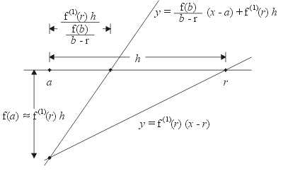
Figure 1. The function f(x) near a and r with one iteration of the false-position method.

The error after one iteration is h minus the width of the smaller shown interval, or:

Therefore, the closer b is to r, the better an approximation f(b)/(b - r) is to the derivative f⁽¹⁾(r), and therefore, the faster the convergence.

To visualize this, suppose the right end point b is fixed and the other, a, is sufficiently close to the root that the function f(x) is closely approximated by the Taylor series, that is, f(a) ≈ f⁽¹⁾(r)(a - r). The lines interpolating the point (a, f(a)) and (b, f(b)) are essentially parallel to the line interpolating (r, 0) and (b, f(b)), which is demonstrated in Figure 2 for the function f(x) = x² - 5 starting with the interval [2, 7].

Figure 2. The secants passing through (a, f(a)) and (5^½, 0).

Thus, focusing in on the region around the root and iterating, we have the behaviour seen in Figure 3 where the next approximation follows a slope which is approximately parallel to the blue line shown in Figure 2. (The aspect ratios of both Figures 2 and 3 are equally distorted.)

Figure 3. Convergence of the false-position method.

Questions

Question 1

Approximate the root of f(x) = x³ - 3 with the false-position method starting with the interval [1, 2] and use ε_step = 0.1 and ε_abs = 0.1 . Use five decimal digits of accuracy.

Answer: 1.4267

Question 2

Approximate the root of f(x) = x² - 10 with the false-position method starting with the interval [3, 4] and use ε_step = 0.1 and ε_abs = 0.1 .

Answer: 3.16

Matlab

The false-position method in Matlab is quite straight-forward. Assume a file f.m with contents

function y = f(x)
   y = x^3 - 2;

exists. Then:

>> format long
>> eps_abs = 1e-5;
>> eps_step = 1e-5;
>> a = 0.0;
>> b = 2.0;
>> step_size = Inf;
>> while (step_size >= eps_step || ( abs( f(a) ) >= eps_abs && abs( f(b) )  >= eps_abs ) )
    c = (f(a)*b - f(b)*a)/(f(a) - f(b));

    if ( f(c) == 0 )
       break;
    elseif ( f(a)*f(c) < 0 )
       step_size = b - c;
       b = c;
    else
       step_size = c - a;
       a = c;
    end
end
>> [a b]
ans = 1.259915864579067   2
>> abs(f(a))
ans =    0.0000246934256663
>> abs(f(b))
ans =    6

Thus, we would choose 1.259915864579067 as our approximation to the cube-root of 2, which has an actual value (to 16 digits) of 1.259921049894873.

An implementation of a function would be

function [ r ] = false_position( f, a, b, N, eps_step, eps_abs )
    % Check that that neither end-point is a root
    % and if f(a) and f(b) have the same sign, throw an exception.

    if ( f(a) == 0 )
	r = a;
	return;
    elseif ( f(b) == 0 )
	r = b;
	return;
    elseif ( f(a) * f(b) > 0 )
        error( 'f(a) and f(b) do not have opposite signs' );
    end

    % We will iterate N times and if a root was not
    % found after N iterations, an exception will be thrown.

    c_old = Inf;

    for k = 1:N
        % Find the false position
        c = (a*f(b) + b*f(a))/(f(b) - f(a));

        % Check if we found a root or whether or not
        % we should continue with:
        %          [a, c] if f(a) and f(c) have opposite signs, or
        %          [c, b] if f(c) and f(b) have opposite signs.

        if ( f(c) == 0 )
            r = c;
            return;
        elseif ( f(c)*f(a) < 0 )
            b = c;
        else
            a = c;
        end

        % If |b - a| < eps_step, check whether or not
        %       |f(a)| < |f(b)| and |f(a)| < eps_abs and return 'a', or
        %       |f(b)| < eps_abs and return 'b'.

        if ( abs( c - c_old ) < eps_step )
            if ( abs( f(a) ) < abs( f(b) ) && abs( f(a) ) < eps_abs )
                r = a;
                return;
            elseif ( abs( f(b) ) < eps_abs )
                r = b;
                return;
            end
        end

	c_old = c;
    end

    error( 'the method did not converge' );
end

Maple

The false-position method in Maple is quite straight-forward:

> epsilon[abs] := 1e-5:
> epsilon[step] := 1e-5:
> f := x -> x^3 - 2:
> a := 0.0:
> b := 2.0:
> step_size := infinity:
> while step_size >= epsilon[step] or ( abs( f(a) ) >= epsilon[abs] and abs( f(b) ) >= epsilon[abs] ) do
    c := (f(a)*b - f(b)*a)/(f(a) - f(b));

    if f(c) = 0 then
       break;
    elif f(a)*f(c) < 0 then
       step_size := b - c;
       b := c;
    else
       step_size := c - a;
       a := c;
    end if;
end do:
> [a, b];
                               [1.259915864, 2.0]

> abs( f(a) );
                                      0.000024696
                        
> abs( f(b) );
                                      6.000

Thus, we would choose 1.259915864 as our approximation to the cube-root of 2, which has an actual value (to 10 digits) of 1.259921050.

Topic 10.2: False-Position Method

Background

References

Theory

Halting Conditions

The Effect of Non-linear Functions

HOWTO

Problem

Assumptions

Tools

Initial Requirements

Iteration Process

Halting Conditions

Examples

Example 1

Example 2

Engineering

Error

Questions

Question 1

Question 2

Matlab

Maple