Topic 10.2: False-Position Method (Error Analysis)

Introduction Notes Theory HOWTO Examples Engineering Error Questions Matlab Maple

The error analysis for the false-position method is not as easy as it is for the bisection method, however, if one of the end points becomes fixed, it can be shown that it is still an O(h) operation, that is, it is the same rate as the bisection method, usually faster, but possibly slower. For differentiable functions, the closer the fixed end point is to the actual root, the faster the convergence.

To see this, let r be the root, and assume that the point b is fixed. Then, the change in a will be proportional to the difference between the slope between (r, 0) and (b, f(b)) and the derivative at r. To view this, first, let the error be h = a - r and assume that we are sufficiently close to the root so that f(a) ≈ f⁽¹⁾(r) h. The slope of the line connecting (a, f(a)) and (b, f(b)) is approximately f(b)/(b - r). This is shown in Figure 1.

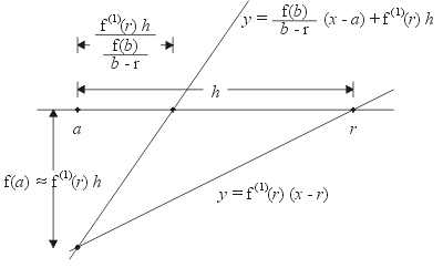
Figure 1. The function f(x) near a and r with one iteration of the false-position method.

The error after one iteration is h minus the width of the smaller shown interval, or:

Therefore, the closer b is to r, the better an approximation f(b)/(b - r) is to the derivative f⁽¹⁾(r), and therefore, the faster the convergence.

To visualize this, suppose the right end point b is fixed and the other, a, is sufficiently close to the root that the function f(x) is closely approximated by the Taylor series, that is, f(a) ≈ f⁽¹⁾(r)(a - r). The lines interpolating the point (a, f(a)) and (b, f(b)) are essentially parallel to the line interpolating (r, 0) and (b, f(b)), which is demonstrated in Figure 2 for the function f(x) = x² - 5 starting with the interval [2, 7].

Figure 2. The secants passing through (a, f(a)) and (5^½, 0).

Thus, focusing in on the region around the root and iterating, we have the behaviour seen in Figure 3 where the next approximation follows a slope which is approximately parallel to the blue line shown in Figure 2. (The aspect ratios of both Figures 2 and 3 are equally distorted.)

Figure 3. Convergence of the false-position method.