Müller's method is a technique for finding the root of a scalar-valued function f(x) of a single variable x when no information about the derivative exists. It is a generalization of the secant method, but instead of using two points, it uses three points and finds an interpolating quadratic polynomial.
This method is better suited to finding the roots of polynomials, and therefore we will focus on this particular application of Müller's method.
Background
Useful background for this topic includes:
- 3. Iteration
- 5. Interpolation
References
- Mathews, Section 2.5, Muller's Method, p.92.
- Weisstein, http://mathworld.wolfram.com/MullersMethod.html.
Theory
Shifting
Given a function f(x) of a single variable, the modified function f(x + T) shifts the function to the left by T. (This will be used extensively in your course on linear systems and signals.) For example, if you examine function f(x) in Figure 1, you will note that the interesting behaviour around the point x = 3 is shifted to the origin by evaluating f(x + 3).
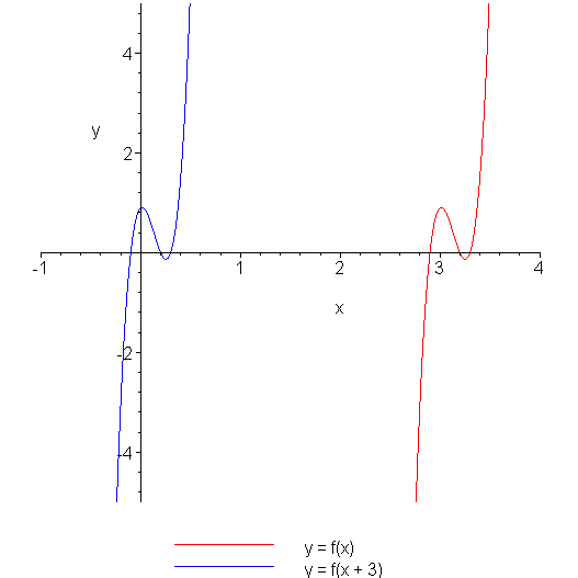
Figure 1. Shifting a function f(x) to the left.
Müller's Method
Given a function p(x), suppose we have three approximations of a root, x1, x2, and x3. Using the Vandermonde method, we can easily find the interpolating quadratic polynomial ax2 + bx + c by solving:
We can then let x4 be a root of this interpolating quadratic polynomial, and this point should be a better approximation of the root than any of x1, x2, or x3. Unfortunately, we run into two problems:
- Which of the two roots do we choose (the larger or the smaller), and
- Which formula do we use to find the root.
You will recall from the example of the quadratic equation where the different forms of the quadratic formula may result in numerically inaccurate values.
For example, consider the points function f(x) (in red) and the interpolating polynomial (in blue) shown in Figure 2.
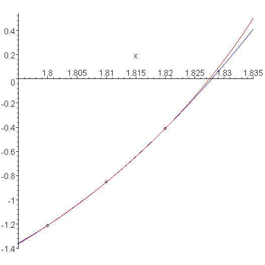
Figure 2. A function p(x) (red), three points, and an interpolating quadratic polynomial (blue).
It appears that the interpolating polynomial is concave up, and therefore we want the larger root. This is made clearer in Figure 3 which plots just the interpolating polynomial.
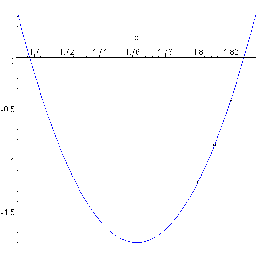
Figure 3. The three points and the interpolating quadratic polynomial.
However, it is apparent that with a slightly different function p(x), we may want the larger root.
To remedy this situation, consider plotting the function p(x - x2), in this example, p(x - 1.81). Because 1.81 is a good approximation to the root, the root of p(x - x2) is now near the origin. This is shown in Figure 4.
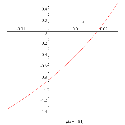
Figure 4. The three points and the interpolating quadratic polynomial.
The interpolating quadratic function will now, similarly have a root near the origin, as is shown in Figure 5.
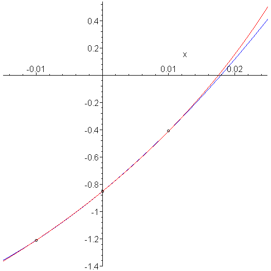
Figure 5. The polynomial interpolating the shifted function.
To emphasize, a plot of the interpolating polynomial indicates quite clearly that we are now interested in the root with the smaller absolute value, as shown in Figure 6.

Figure 6. The interpolating polynomial.
Thus, if the interpolating polynomial is ax2 + bx + c, we must use the formula
Note, this gives us the root of the shifted function p(x + 1.81). If we want the root of the quadratic function in Figure 2, we must add 1.81 back onto the value of this root.
When the coefficient b and the discriminant b2 − 4ac ≥ 0, then to maximize the denominator, we need only choose the sign equal to the sign of b, that is use
Suppose, however, that these are not real. In this case, we must be more careful. Let b = br + jbj and let the square root of the discriminant be represented by d = dr + jdj. Thus, the norm of b ± d are
br2 − 2brdr + dr2 + bj2 − 2bjdj + dj2
Thus, to maximize this, we must choose whichever sign makes brdr + bjdj positive. In the case where this sum is zero, then either:
- We are at a root, or
- One of b and d is real, the other imaginary. In this case, choose whichever makes d negative.
The second case ensures that we are always finding a root with a positive imaginary part. There is no mathematical benefit to this, it is simply a choice.
HOWTO
Problem
Given a polynomial of one variable, p(x), find a value r (called a root) such that p(r) = 0.
Assumptions
This method will work for non-polynomial functions, but it is more appropriate for finding the roots of polynomials due to its ability to jump from real to complex iterates.
Tools
We will use sampling, quadratic interpolation, and iteration.
Initial Requirements
We have three initial approximation x0, x1, and x2 of the root. It would be useful if |f(x0)| > |f(x1)| > |f(x2)|, that is, the points are in descending absolute value when evaluated by f.
Iteration Process
Given three approximation xn - 2, xn - 1, and xn, can find an interpolating quadratic polynomial which passes through the points:
- (xn − 2 − xn − 1, f(xn − 2))
- (0, f(xn − 1))
- (xn − xn − 1, f(xn))
In this case, it is easiest (and numerically stable) to use the Vandermonde method to find the interpolating quadratic polynomial ax2 + bx + c:
Having found the coefficients of the interpolating polynomial, we may now choose to find the root. There are two formulae for finding the roots of a quadratic polynomial: one with the radical in the numerator, the other with the radical in the denominator:
and
Because we are assuming that the three points xn - 2, xn - 1, and xn are good approximations to the root, it follows that we want to find the root closest to these points, that is, the smallest root of the polynomial we found. The second formula is more numerically stable for finding the smallest root of a quadratic polynomial, and therefore we set:
where the sign in the denominator is equal to the sign of b.
Halting Conditions
There are three conditions which may cause the iteration process to halt (these are the same as the halting conditions for Newton's method):
- We halt if both of the following conditions are met:
- The step between successive iterates is sufficiently small, |xn + 1 - xn| < εstep, and
- The function evaluated at the point xn + 1 is sufficiently small, |f(xn + 1)| < εabs.
- If the system does not have a solution, we halt.
- If we have iterated some maximum number of times, say N, and have not met Condition 1, we halt and indicate that a solution was not found.
If we halt due to Condition 1, we state that xn + 1 is our approximation to the root.
If we halt due to either Condition 2 or 3, we may either choose a different initial approximations x0 and x1, or state that a solution may not exist.
Examples
Example 1
Suppose we wish to find a root of the polynomial f(x) = x7 + 3x6 + 7x5 + x4 + 5x3 + 2x2 + 5x + 5. There exist closed form solutions to the roots of polynomials for quartics and below, and this is a degree seven polynomial, so thus we must use a numerical technique. We will use x0 = 0, x1 = -0.1, and x2 = -0.2 as our three initial approximations. We will let the two values εstep = 0.0001 and εabs = 0.0001 and we will halt after N = 100 iterations.
We will use six decimal digit arithmetic to find a solution.
The easiest way to present such information is in tabular format:
| n | xn - 2 | xn - 1 | xn | xn + 1 | |f(xn + 1)| | |xn + 1 - xn| |
|---|---|---|---|---|---|---|
| 2 | 0.0 | -0.1 | -0.2 | -1.14874 | 13.6910 | 0.94874 |
| 3 | -0.1 | -0.2 | -1.14874 | -0.568100 | 1.65995 | 0.580640 |
| 4 | -0.2 | -1.14874 | -0.568100 | -0.669622 | 0.51613 | 0.101522 |
| 5 | -1.14874 | -0.568100 | -0.669622 | -0.702849 | 0.05806 | 0.033227 |
| 6 | -0.568100 | -0.669622 | -0.702849 | -0.706858 | 0.00047 | 0.004009 |
| 7 | -0.669622 | -0.702849 | -0.706858 | -0.706826 | 0.00001 | 0.000032 |
Thus, with the last step, both halting conditions are met, and therefore, after six iterations, our approximation to the root is -0.706826 .
Example 2
The following demonstrates the first six iterations of Müller's method in Matlab. Suppose we wish to find a root of the same polynomial
starting with the same three initial approximations x0 = 0, x1 = -0.1, and x2 = -0.2.
The first formula in red is the root of the quadratic polynomial which is added onto the middle approximation x(2).
>> p = [1 3 7 1 5 2 5 5]
p =
1      3      7      1      5      2      5      5

>> x = [0.0 -0.1 -0.2]'      % first three approximations
x =
   0.00000
  -0.10000
  -0.20000

>> % 1st iteration ---------------------------------------
>> M = [(x(1) - x(2))^2,  x(1) - x(2),  1
      0,               0,       1
(x(3) - x(2))^2,  x(3) - x(2),  1]
M =
   0.01000   0.10000   1.00000
   0.00000   0.00000   1.00000
   0.01000  -0.10000   1.00000

>> y = polyval( p, x )
y =
  5.00000
  4.51503
  4.03954

>> c = M \ y
c =
  0.47367
  4.80230
  4.51503

>> x = [x(2), x(3), x(2) - 2*c(3)/(c(2) + sqrt(c(2)^2 - 4*c(1)*c(3)))]'
x =
  -0.10000
  -0.20000
  -1.14864

>> % 2nd iteration ---------------------------------------
>> M = [(x(1) - x(2))^2,  x(1) - x(2),  1
      0,               0,       1
(x(3) - x(2))^2,  x(3) - x(2),  1]
M =
   0.01000   0.10000   1.00000
   0.00000   0.00000   1.00000
   0.89992  -0.94864   1.00000

>> y = polyval( p, x )
y =
    4.5150
    4.0395
  -13.6858

>> c = M \ y
c =
  -13.2838
    6.0833
    4.0395

>> x = [x(2), x(3), x(2) - 2*c(3)/(c(2) + sqrt(c(2)^2 - 4*c(1)*c(3)))]'
x =
  -0.20000
  -1.14864
  -0.56812

>> % 3rd iteration ---------------------------------------
>> M = [(x(1) - x(2))^2,  x(1) - x(2),  1
      0,               0,       1
(x(3) - x(2))^2,  x(3) - x(2),  1]
M =
  0.89992  0.94864  1.00000
  0.00000  0.00000  1.00000
  0.33701  0.58052  1.00000

>> y = polyval( p, x )
y =
    4.0395
  -13.6858
    1.6597

>> c = M \ y
c =
  -21.0503
   38.6541
  -13.6858

>> x = [x(2), x(3), x(2) - 2*c(3)/(c(2) + sqrt(c(2)^2 - 4*c(1)*c(3)))]'
x =
  -1.14864
  -0.56812
  -0.66963

>> % 4th iteration ---------------------------------------
>> M = [(x(1) - x(2))^2,  x(1) - x(2),  1
      0,               0,       1
(x(3) - x(2))^2,  x(3) - x(2),  1]
M =
   0.33701  -0.58052   1.00000
   0.00000   0.00000   1.00000
   0.01030  -0.10151   1.00000

>> y = polyval( p, x )
y =
  -13.6858
    1.6597
    0.5160

>> c = M \ y
c =
  -31.6627
    8.0531
    1.6597

>> x = [x(2), x(3), x(2) - 2*c(3)/(c(2) + sqrt(c(2)^2 - 4*c(1)*c(3)))]'
x =
  -0.56812
  -0.66963
  -0.70285

>> % 5th iteration ---------------------------------------
>> M = [(x(1) - x(2))^2,  x(1) - x(2),  1
      0,               0,       1
(x(3) - x(2))^2,  x(3) - x(2),  1]
M =
   0.01030   0.10151   1.00000
   0.00000   0.00000   1.00000
   0.00110  -0.03322   1.00000

>> y = polyval( p, x )
y =
  1.65973
  0.51602
  0.05802

>> c = M \ y
c =
  -18.6991
   13.1653
    0.5160

>> x = [x(2), x(3), x(2) - 2*c(3)/(c(2) + sqrt(c(2)^2 - 4*c(1)*c(3)))]'
x =
  -0.66963
  -0.70285
  -0.70686

>> % 6th iteration ---------------------------------------
>> M = [(x(1) - x(2))^2,  x(1) - x(2),  1
      0,               0,       1
(x(3) - x(2))^2,  x(3) - x(2),  1]
M =
   0.00110   0.03322   1.00000
   0.00000   0.00000   1.00000
   0.00002  -0.00401   1.00000

>> y = polyval( p, x )
y =
   0.51602
   0.05802
  -0.00046

>> c = M \ y
c =
  -21.8018
   14.5107
    0.0580

>> x = [x(2), x(3), x(2) - 2*c(3)/(c(2) + sqrt(c(2)^2 - 4*c(1)*c(3)))]'
x =
  -0.70285
  -0.70686
  -0.70683
The list of all iterations using Matlab are:
   0.000000000000000
  -0.100000000000000
  -0.200000000000000
  -1.148643697414111
  -0.568122032631211
  -0.669630566165950
  -0.702851144883234
  -0.706857484921269
  -0.706825973130949
  -0.706825980788168
  -0.706825980788170
Note how convergence speeds up after none of the first three initial approximations are used to calculate the next iterate?
Engineering
As mentioned in the the engineering application of polynomials, finding the roots of a polynomial are necessary when determining the behaviour and stability of a linear system.
Error
The error analysis for Müller's method is beyond the scope of this course, but it can be shown to be O(hp) where p ≈ 1.839286755. This rate of convergence is faster than the secant method but slower than Newton's method.
It can be shown that the power p is the real root of the cubic x3 − x3 − x − 1, that is, p = (a + 4/a + 1)/3 where a = (19 + 3√33)1/3.
Example
To demonstrate this, we will find the root of f(x) = x − x3/3 starting with the three points x0 = 1, x1 = 0.75, x2 = 0.5 and iterate to find:
|
1.0 7.5e-1 5.0e-1 8.4560e-2 9.1422e-3 1.2683e-4 3.2675e-8 1.2629e-14 1.7447e-26 2.3999e-48 1.7626e-88 2.4601e-162 3.4688e-298 |
Because again the root is at the origin, the approximation equals the error, and thus, if we find the best fitting least-squares line through the points (ln(hk), ln(hk + 1)) for k = 0, ..., 12, we get -0.45559 + 1.83936h. The points and the best fitting least-squares line are shown in Figure 1.
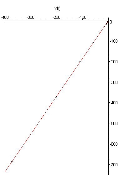
Figure 1. The points (ln(hk), ln(hk + 1)) and the best fitting least-squares line.
Again, an example is not a proof, but it supports and demonstrates the propostion.
Questions
Question 1
Using Matlab, perform four iterations of finding a root of the polynomial p(x) = x3 + 3x2 + 5x - 7 starting with the points x0 = 1, x1 = 2, x3 = 3.
Question 1
Using Matlab, perform four iterations of finding a root of the polynomial p(x) = x4 + 3x3 + 5x - 7 starting with the points x0 = 1, x1 = 2, x3 = 3.
Question 3
Given the polynomial p = [2 3 5 2 1], the roots are approximately
First use deconv to divide out the first root, and then use it again on the answer to divide out the second root. Compare this to the answer when you divide out the product of the roots with deconv( p, [1 1.11572 1.79227] ). (We get the second from the formula (x - z)(x - z*) = x2 - 2ℜ(z) + |z|2).
Matlab
Implementing Müller's method in Matlab is not that difficult:
eps_step = 1e-5;
eps_abs = 1e-5;
p = [1 2 3 4 2];
x = [0 -0.1 -0.2]';
y = polyval( p, x );
while ( true )
     V = vander( x - x(2) );
     c = V \ y;
     disc = sqrt( c(2)^2 - 4*c(1)*c(3) );

     % if ( real(c(2))*real(disc) + imag(c(2))*imag(disc) > 0 )

     if abs( c(2) + disc ) > abs( c(2) - disc )
         denom = c(2) + disc;
     else
         denom = c(2) - disc;
     end

     [roots(c)', -2*c(3)/denom, x'];

     x = [x(2), x(3), x(2) - 2*c(3)/denom]';

     y = [y(2), y(3), polyval( p, x(3) )]';

     if ( abs( x(2) - x(3) ) < eps_step && abs( y(3) ) < eps_abs )
        break;
     end
end
x(3)
Maple
Implementing Müller's method in Maple is not that difficult:
To be completed...
> eps_step := 1e-5;
> eps_abs := 1e-5;
> p := x -> x^4 + 2*x^3 + 3*x^2 + 4*x - 7;
> x = <0, -0.1, -0.2>;
> y = map( p, x );
> for i from 1 to 100 do
     V = vander( x - x(2) );
     c = V \ y;
     x = ;

     if abs( x[2] - x[3] ) < eps_step and abs( y[3] ) < eps_abs  then
	break;
     elif ( i == 100 )
        error ( 'Muller\'s method failed to converge' );
     end if;
 end do;
>> x(3)
Copyright ©2005 by Douglas Wilhelm Harder. All rights reserved.


