Introduction Notes Theory HOWTO Examples Engineering Error Questions Matlab Maple

Shifting

Given a function f(x) of a single variable, the modified function f(x + T) shifts the function to the left by T. (This will be used extensively in your course on linear systems and signals.) For example, if you examine function f(x) in Figure 1, you will note that the interesting behaviour around the point x = 3 is shifted to the origin by evaluating f(x + 3).

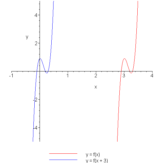
Figure 1. Shifting a function f(x) to the left.

Müller's Method

Given a function p(x), suppose we have three approximations of a root, x₁, x₂, and x₃. Using the Vandermonde method, we can easily find the interpolating quadratic polynomial ax² + bx + c by solving:

We can then let x₄ be a root of this interpolating quadratic polynomial, and this point should be a better approximation of the root than any of x₁, x₂, or x₃. Unfortunately, we run into two problems:

Which of the two roots do we choose (the larger or the smaller), and
Which formula do we use to find the root.

You will recall from the example of the quadratic equation where the different forms of the quadratic formula may result in numerically inaccurate values.

For example, consider the points function f(x) (in red) and the interpolating polynomial (in blue) shown in Figure 2.

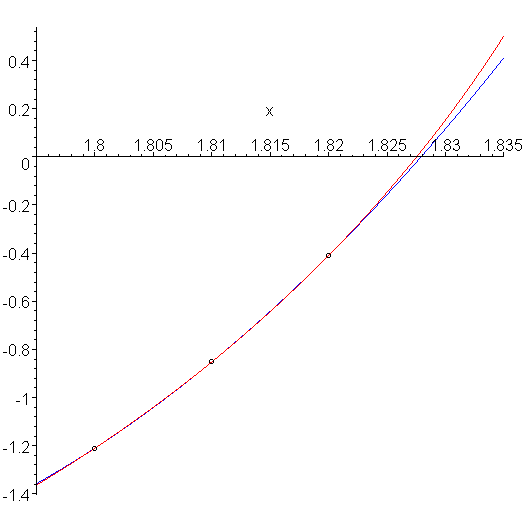
Figure 2. A function p(x) (red), three points, and an interpolating quadratic polynomial (blue).

It appears that the interpolating polynomial is concave up, and therefore we want the larger root. This is made clearer in Figure 3 which plots just the interpolating polynomial.

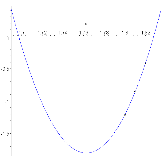
Figure 3. The three points and the interpolating quadratic polynomial.

However, it is apparent that with a slightly different function p(x), we may want the larger root.

To remedy this situation, consider plotting the function p(x - x₂), in this example, p(x - 1.81). Because 1.81 is a good approximation to the root, the root of p(x - x₂) is now near the origin. This is shown in Figure 4.

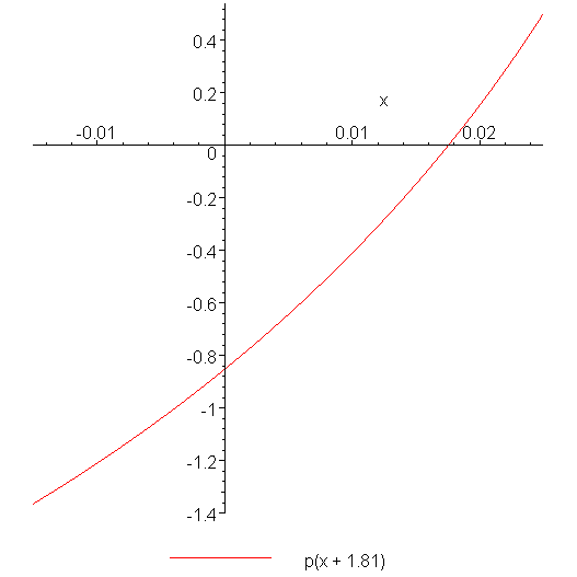
Figure 4. The three points and the interpolating quadratic polynomial.

The interpolating quadratic function will now, similarly have a root near the origin, as is shown in Figure 5.

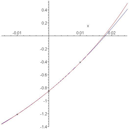
Figure 5. The polynomial interpolating the shifted function.

To emphasize, a plot of the interpolating polynomial indicates quite clearly that we are now interested in the root with the smaller absolute value, as shown in Figure 6.

Figure 6. The interpolating polynomial.

Thus, if the interpolating polynomial is ax² + bx + c, we must use the formula

Note, this gives us the root of the shifted function p(x + 1.81). If we want the root of the quadratic function in Figure 2, we must add 1.81 back onto the value of this root.

When the coefficient b and the discriminant b² − 4ac ≥ 0, then to maximize the denominator, we need only choose the sign equal to the sign of b, that is use

Suppose, however, that these are not real. In this case, we must be more careful. Let b = b_r + jb_j and let the square root of the discriminant be represented by d = d_r + jd_j. Thus, the norm of b ± d are

b_r² + 2b_rd_r + d_r² + b_j² + 2b_jd_j + d_j²
b_r² − 2b_rd_r + d_r² + b_j² − 2b_jd_j + d_j²

Thus, to maximize this, we must choose whichever sign makes b_rd_r + b_jd_j positive. In the case where this sum is zero, then either:

We are at a root, or
One of b and d is real, the other imaginary. In this case, choose whichever makes d negative.

The second case ensures that we are always finding a root with a positive imaginary part. There is no mathematical benefit to this, it is simply a choice.

Topic 10.6: Müller's Method (Theory)

Shifting

Müller's Method