Using points on either side of a point x0 results in the best approximations of the derivative. Unfortunately, often in engineering, especially in real-time applications, we must use only past data to estimate the derivative at a point. For example, it may be necessary to use the current rate-of-change of an incoming signal to adjust a system, but only past points are available. Formula which use a technique similar to that in 13.1 and use only points ≤ x0 to approximate the derivative at x0 are termed backward divided-difference formula.
There are corresponding formulae using points greater than or equal to x0, but the derivation of these are left as an exercise to the reader.
Background
Useful background for this topic includes:
References
- Bradie, Section 6.2, Numerical Differentiation, Part II, p.438.
- Mathews, Section 6.2, Numerical Differentiation Formulas, p.343.
- Chapra, Section 23.1, High-accuracy Differentiation Formaulas, p.634.
Interactive Maplet
To generate a backward divided-difference formula, keep the points to the left of x, for example, f(x - 3*h) to f(x).
Theory
Suppose you want to approximate the derivative of a function f(x) at a point x0. Given a small value of h, then if we can evaluate the function to find the two points (x0 − h, f(x0 − h)) and (x0, f(x0)) then we can find the interpolating polynomial passing through these points. For example, Figure 1 shows a function and a point at which we would like to approximate the derivative. Figure 2 shows how we can approximate the derivative by finding an interpolating linear polynomial.
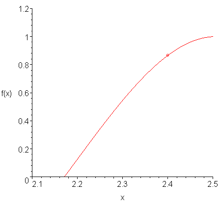
Figure 1. A function f(x).
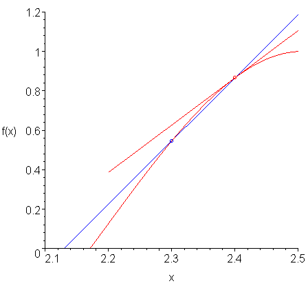
Figure 2. A function f(x) and a linear interpolating polynomial approximating the derivative.
Similarly, if we can evaluate the function at three points (x0 − 2h, f(x0 − 2h)), (x0 − h, f(x0 − h)), and (x0, f(x0)), then we can find the interpolating polynomial passing through these points.
If we let h = 0.1, then we can calculate the three points shown in Figure 3 and find the interpolating quadratic polynomial.
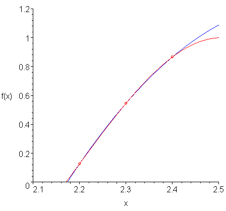
Figure 3. The line tangent to the point (xa, f(xa)).
Figure 4 shows this interpolating quadratic polynomial and the slope at the point x = 2.4. This is easily calculated, as the quadratic is of the form ax2 + bx + c and thus, the slope at x = 2.4 is 2a⋅2.4 + b.
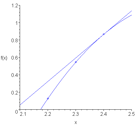
Figure 4. The slope of the interpolating quadratic polynomial at x = 2.4.
If we compare the approximation of the slope found using the interpolating quadratic polynomial and the actual slope at x = 2.4, we see that in Figure 5 that they are close, but not exactly the same.
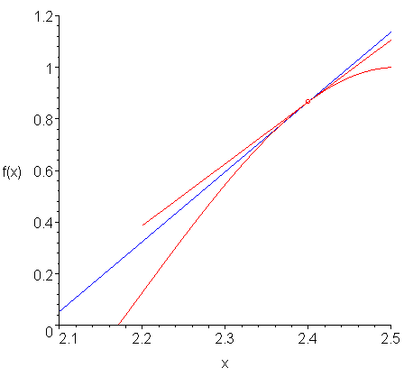
Figure 5. A comparison of the two slopes.
Derivation
Because we are considering points to the left of x0, these methods are termed backward divided difference.
We will look at two formulae, interpolating two and three points, respectively. Beyond this, the instability of the interpolating polynomials reduces the benefit of finding higher and higher order formulae.
First-Order Backward Divided-Difference Formula
Interpolating the two points (x0 − h, f(x0 − h)) and (x0, f(x0)), differentiating and evaluating at x0 yields the familiar formula
Second-Order Backward Divided-Difference Formula
Interpolating the three points (x0 − 2h, f(x0 − 2h)), (x0 − h, f(x0 − h)), and (x0, f(x0)), differentiating and evaluating at x0 yields the formula
If you wish to see the derivation of these formulae, please look at this Maple worksheet.
Higher-Order Backward Divided Difference Formula
It is possible to find polynomials which interpolate four or more points, but you should recall that interpolating polynomials are subject to polynomial wiggle which has a greater effect closer to the end points. Consequently, the formulae are not very exact; the error term for the n-point backward divided-difference formula is given by:
Note that the coefficient 1/n does not grow as quickly as the coefficient of the centred-divided difference formulae, which follow 1/6, 1/30, 1/630, 1/2772, 1/12012, 1/51480, 1/218790,
HOWTO
Problem
Approximate the derivative of a univariate function f(x) at a point x0. We will assume that we are given a sequence of points (xi, f(xi)). We will not look at iteration because the process of Richardson extrapolation is significantly better.
Assumptions
We need to assume the function has a second derivative if we are to bound the error on our approximation.
Tools
We will use interpolation.
Process
If we are to evaluate the derivative at the point (xi, f(xi)) and have access to previous point (xi − 1, f(xi − 1)) then we may calculate:
This is simply another form of the formula
where h is the distance between the points, that is, h = xi - xi − 1.
If we have access to two previous points of xi, we can calculate
where h = xi - xi − 1.
This is another form of the formula:
Examples
Example 1
Given the data points ..., 3.2, 3.3, 3.4, 3.5, 3.6, ... which measure the rotation of a satellite dish at points in time, with angles 1.05837 1.15775 1.25554 1.35078 1.44252, approximate the rate of change of the angle at time 3.4 using both the 1st-order and 2nd-order backward divided-difference formulae.
(1.25554 − 1.15775)/0.1 = 0.9779 and (1.05837 − 4⋅1.15775 + 3⋅1.25554)/(2⋅0.1) = 0.970285.
Thus, 0.970285 is the more accurate answer. The data was taken from a curve which has an exact derivative of 0.96680 at 3.4.
Engineering
To be completed.
Error
1st-Order Backward Divided-Difference Formula
To determine the error for the 1st-order backward divided-difference formula, we need only look at the Taylor series approximation:
Simply rearranging and dividing by h yields the formula:
Thus, the error is O(h).
2nd-Order Backward Divided-Difference Formula
To determine the error for the 2nd-order backward divided-difference formula, we need only look at the two Taylor series approximations:
and subtract the first from 4× the second, and rearrange, we get the that:
Note that the sum of the coefficients in the parentheses is 1, and therefore may be approximated by the average of f(3)(x) on the interval [x - 2h, x], and therefore the formula is O(h2).
Compare the error of the 2nd-order formula to that using the error of the 2nd-order centred divided-difference formula which has a coefficient -1/6, and thus, the centred divided-difference formula has, approximately, half the absolute error of the backward divided-difference formula. To view this, consider Figure 1. Here we see the points used to approximate the 2nd-order backward (black) and centred (blue) divided-difference formulae to approximate the derivative (magenta) at the fixed point. You will note that the error of the centred approximation is approximately half that of the backward approximation.
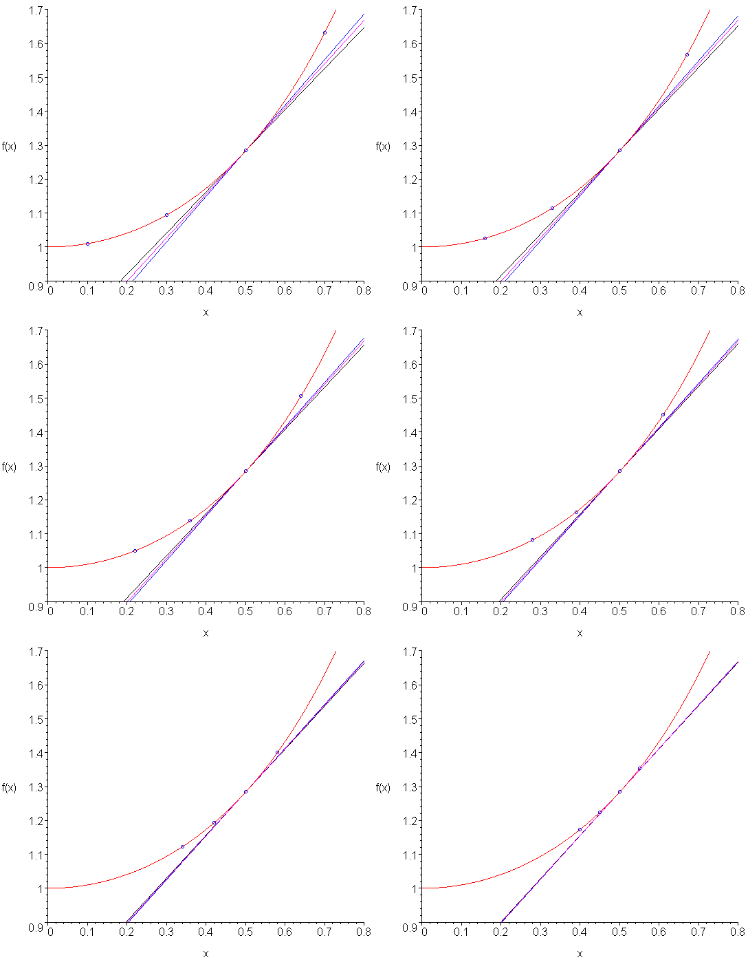
Figure 1. Comparison of 2nd-order centred and backward divided-difference approximations of the derivative.
The function shown in Figure 1 is f(x) = exp( x2 ) and the point is x = 0.5 . Table 1 shows the approximations and the errors for h = 0.1 and h = 0.01. The actual derivative at that point is 1.284025417.
Table 1. Comparison of errors.
| h | Centred | Centred error | Backward | Backward error |
|---|---|---|---|---|
| 0.1 | 1.2991 | 0.0151 | 1.2610 | 0.023 |
| 0.01 | 1.2842 | 0.00015 | 1.2837 | 0.00029 |
You will notice that the error of the centred divided-difference formula is approximately half that of the backward divided-difference formula. Additionally, both errors in the second row are approximately 0.12 = 0.01 that of the first row.
Questions
Question 1
Approximate the current at the midpoint of the incoming data ..., 7.2, 7.3, 7.4, 7.5, 7.6, ... where the charge on a capacitor these times is 0.00242759 0.00241500 0.00240247 0.00239001 0.00237761.
Answer: -0.0001253 and -0.0001250.
Question 2
Note that the coefficients in the numerator and denominator add up to zero. (-1 + 1 = 1 - 4 + 3 = 0). What would happen if these did not add up to zero?
Answer: Consider what would happen if added, for example, 5, to each of the y values.
Matlab
In Matlab, you would approximate the derivative numerically:
>> ( sin( 1.5 ) - sin( 1.3 ) )/0.2
which would approximate the actual derivative of cos(1.5).
Maple
Maple calculates derivatives symbolically:
> diff( sin(x), x );
                             cos(x)
For more help on the diff routine, enter:
?diff
Copyright ©2005 by Douglas Wilhelm Harder. All rights reserved.


