

Up to now, we have seen three techniques for reducing the error for solving an initial value problem of the form:
y(a) = y0
where we estimated for y(b) with a single step (or iteration). To get a better answer, use the same strategy as we did for the composite trapezoidal rule by breaking the interval up into smaller sub intervals and applying either Euler's, Heun's or the 4th-order Runge Kutta methods on each subinterval.
Background
Useful background for this topic includes:
- 4. Linear Algebra
- 14.1 Euler's Method
- 14.2 Heun's Method
- 14.3 4th-Order Runge-Kutta Method
References
See the corresponding references in the last three background topics.
Theory
Given the IVP
y(a) = y0
where we want to estimated y(b) for b > a, we can apply the same strategy we used for the composite-trapezoidal rule:
Break the interval [a, b] into n sub-intervals and define h = (b - a)/n. Then set ti = a + ih for i = 0, 1, ..., n. Therefore t0 = a and tn = b.
Now, y0 is the initial value so let yi represent the approximation of y(ti) for i = 1, 2, ..., n.
Using any of the three techniques we've seen, Euler's, Heun's, or 4th-order Runge Kutta, we may now proceed as follows:
For i from 1 to n:
Approximate yi using yi − 1.
More specifically:
Multiple-step Euler's Method
Calculate
for i = 1, 2, ..., n.
Multiple-step Heun's Method
Calculate
K0 = f(ti − 1, yi − 1)
K1 = f(ti, yi − 1 + h K0)
and set yi = yi − 1 + h (K0 + K1)/2.
4th-order Runge Kutta
Calculate
K0 = f(ti − 1, yi − 1)
K1 = f(ti − 1 + ½h, yi − 1 + ½h K0)
K2 = f(ti − 1 + ½h, yi − 1 + ½h K1)
K3 = f(ti, yi − 1 + h K2)
and set yi = yi − 1 + h (K0 + 2 K1 + 2 K2 + K3)/6.
HOWTO
Problem
Given the IVP
y(a) = y0
approximate y(b).
Assumptions
The function f(t, y) should be continuous in both variables.
Tools
We will use Taylor series and iteration.
Initial Conditions
Choose a value of n ≥ 1. Set h = (b − a)/n.
Set ti = a + ih for i = 0, 1, ..., n and let yi be the approximation of y(ti) for i = 1, ..., n.
Process
Multiple-step Euler's Method
For i = 1, 2, ..., n set
Multiple-step Heun's Method
For i = 1, 2, ..., n calculate
K0 = f(ti − 1, yi − 1)
K1 = f(ti, yi − 1 + h K0)
and set yi = yi − 1 + h (K0 + K1)/2.
4th-order Runge Kutta
For i = 1, 2, ..., n calculate
K0 = f(ti − 1, yi − 1)
K1 = f(ti − 1 + ½h, yi − 1 + ½h K0)
K2 = f(ti − 1 + ½h, yi − 1 + ½h K1)
K3 = f(ti, yi − 1 + h K2)
and set yi = yi − 1 + h (K0 + 2 K1 + 2 K2 + K3)/6.
Approximating Intermediate Values
If a value of y(t) is required for a < t < b where t ≠ ti for any i, choose the surrounding four points (three if t < t1 or t > tn − 1), find the interpolating polynomial and evaluate this polynomial at the point t. Alternatively, calculate the appropriate cubic spline where the derivatives at the end points are given by f(a, y0) and f(b, yn), respectively.
Examples
Example 1
Perform four steps of each of Euler's method, Heun's method, and 4th-order Runge Kutta on the IVP
y(1)(t) = y(t) t + t - 1
y(0) = 1
In this case, the function f(t, y) = y t + t - 1. Let h = (1 - 0)/4 = 0.25 and thus t0 = 0, t1 = 0.25, t2 = 0.5, t3 = 0.75, t4 = 1 and y0 = 1. Then
Euler's method
y1 = y0 + h f(t0, y0) = 0.75
y2 = y1 + h f(t1, y1) = 0.609375
y3 = y2 + h f(t2, y2) = 0.560546875
y4 = y3 + h f(t3, y3) = 0.603149414
Heun's method
K0 = f(t0, y0) = -1
K1 = f(t0 + h, y0 + h K0) = -0.5625000000
y1 = y0 + ½ h (K0 + K1) = 0.8046875000
K0 = f(t1, y1) = -0.5488281250
K1 = f(t1 + h, y1 + h K0) = -0.1662597656
y2 = y1 + ½ h (K0 + K1) = 0.7153015137
K0 = f(t2, y2) = -0.1423492432
K1 = f(t2 + h, y2 + h K0) = 0.259785652
y3 = y2 + ½ h (K0 + K1) = 0.7299810648
K0 = f(t3, y3) = 0.297485799
K1 = f(t3 + h, y3 + h K3) = 0.804352515
y4 = y3 + ½ h (K0 + K1) = 0.8677108540
4th-order Runge Kutta
K0 = f(t0, y0) = -1
K1 = f(t0 + ½h, y0 + ½hK0) = -0.7656250000
K2 = f(t0 + ½h, y0 + ½hK1) = -0.7619628906
K3 = f(t0 + h, y0 + hK0) = -0.5476226806
y1 = y0 + h (K0 + 2 K1 + 2 K2 + K3)/6 = 0.8082167307
K0 = f(t1, y1) = -0.5479458173
K1 = f(t1 + ½h, y1 + ½hK0) = -0.3476036862
K2 = f(t1 + ½h, y1 + ½hK1) = -0.3382126488
K3 = f(t1 + h, y1 + hK0) = -0.1381682158
y2 = y1 + h (K0 + 2 K1 + 2 K2 + K3)/6 = 0.7224772847
K0 = f(t2, y2) = -0.1387613576
K1 = f(t2 + ½h, y2 + ½hK0) = 0.065707572
K2 = f(t2 + ½h, y2 + ½hK1) = 0.081681707
K3 = f(t2 + h, y2 + hK0) = 0.307173284
y3 = y2 + h (K0 + 2 K1 + 2 K2 + K3)/6 = 0.7417768882
K0 = f(t3, y3) = 0.306332666
K1 = f(t3 + ½h, y3 + ½hK0) = 0.557559912
K2 = f(t3 + ½h, y3 + ½hK1) = 0.585037893
K3 = f(t3 + h, y3 + hK0) = 0.888036361
y4 = y3 + h (K0 + 2 K1 + 2 K2 + K3)/6 = 0.8867587481
The correct answer is y(1) = 0.8867564079.
The plot of the solution and the field plot are shown in Figure 1.
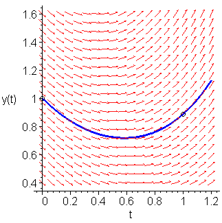
Figure 1. The field plot and the solution.
The approximations are shown in Figure 2.
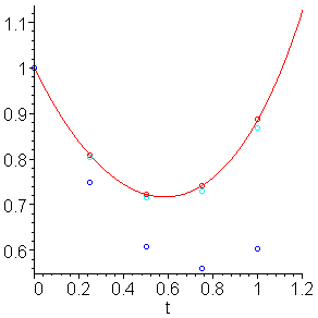
Figure 2. The solution and the three approximations: Euler (blue), Heun (light blue), and 4th-order Runge Kutta (red)
Engineering
To be completed.
Error
Consider the IVP
y(a) = y0
where we are trying to approximate y(b). If we apply Euler's method with n steps, then the error on the ith interval is given by ½y(2)(τi)h2 where τi ∈ [ti − 1, ti]. Thus, the cumulative error is:
If we factor out a ½h and rewrite the other h as (b - a)/n, then we get:
Using the definition of the average value, this simplifies to:
Thus, we can easily generalize this result to see that multiple-step methods will reduce the order of the error term by a factor of h. Thus, while a single step of 4th-order Runge Kutta is O(h5), multiple applications of 4th-order Runge Kutta is only O(h4). (Hence the name, 4th-order Runge Kutta.) A summary is shown in Table 1.
Table 1. Comparison of rates of convergence for single step and multiple steps.
| Method | Single Step | Multiple Steps |
|---|---|---|
| Euler's method | O(h2) | O(h) |
| Heun's method | O(h3) | O(h2) |
| 4th-order Runge Kutta | O(h5) | O(h4) |
This suggests very strongly that it is that much more important to use the 4th-order Runge Kutta method when using multiple step methods.
To justify this statement, let us look at how the error decreases as the size of the interval is increased. We cannot, however, simply divide the interval into n sub-intervals and apply each method because Euler's method requires only one function evaluation, and 4th-order Runge Kutta requires four. Thus, Tables 1, 2, 3, and 4 look at how the error is reduced with a constant number of function evaluations.
Table 1. Four function evaluations.
| Method | Steps | Error Reduction |
|---|---|---|
| Euler's | 4 | 1/4 = 0.25 |
| Heun's | 2 | 1/22 = 0.25 |
| 4th-order Runge Kutta | 1 | 1 |
Table 2. Eight function evaluations.
| Method | Steps | Error Reduction |
|---|---|---|
| Euler's | 8 | 1/8 = 0.125 |
| Heun's | 4 | 1/42 = 0.0625 |
| 4th-order Runge Kutta | 2 | 1/24 = 0.0625 |
Table 3. Sixteen function evaluations.
| Method | Steps | Error Reduction |
|---|---|---|
| Euler's | 16 | 1/16 = 0.0625 |
| Heun's | 8 | 1/82 = 0.0156 |
| 4th-order Runge Kutta | 4 | 1/44 = 0.00391 |
Table 4. Thirty-two function evaluations.
| Method | Steps | Error Reduction |
|---|---|---|
| Euler's | 32 | 1/32 = 0.03125 |
| Heun's | 16 | 1/162 = 0.00391 |
| 4th-order Runge Kutta | 8 | 1/84 = 0.000244 |
Thus, while Euler's method with 32 sub-intervals and 4th-order Runge Kutta with 8 intervals both have the same number of evaluations, the error with Euler's method is reduced by only 0.03125 while the error with 4th-order Runge Kutta is reduced by 0.000244.
To visualize this, consider:
y(1)(t) = 1 + y2(t)
y(0) = 0
The correct answer is y(1) = tan(1) = 1.557407725.
With Euler's method, using four steps, we have:
y1 = 0.25
y2 = 0.515625
y3 = 0.8320922852
y4 = 1.255186678
The absolute error of this answer is 0.30.
With one step of 4th-order Runge Kutta, we have:
y1 = 1.535847982
The absolute error here is 0.022.
If however, we use 32 function evaluations, we have y32 = 1.497473902 which has an absolute error of 0.060 which is approximately 1/5 the error with 4 intervals.
With 8 steps of 4th-order Runge Kutta, we get that y8 = 1.557402847 which has an absolute error of 0.0000049 which is approximately 0.00022 that of the approximation with one step.
Questions
Question 1
Given the IVP
y(0) = 1
approximate y(1) using four steps of Euler's method, Heun's method, and 4th-order Runge Kutta.
Answer: 1.754495239, 1.755786729, 1.755760161
Question 2
Given the same ODE as in Question 1, but with the initial condition y(1) = 2, approximate y(2.0).
Answer: 2.708990479, 2.711573457, 2.711520324
Matlab
To be completed later.
Maple
Given the IVP y(1)(t = t y(t) - t2 + 1 with y(a) = 3, to approximate y(b) with n steps, we can do:
Euler's Method
h := (b - a)/n;
for i from 0 to n do
   t[i] := a + i*h;
end;
y[0] := 3;
f := (t, y) -> t*y - t^2 + 1;
for i from 1 to n do
    y[i] := y[i - 1] + h*f(t[i - 1], y[i - 1]);
end do;
y[n];   # approximation
Heun's Method
h := (b - a)/n;
for i from 0 to n do
   t[i] := a + i*h;
end;
y[0] := 3;
f := (t, y) -> t*y - t^2 + 1;
for i from 1 to n do
    K[0] := f(t[i - 1], y[i - 1]);
    K[1] := f(t[i - 1] + h, y[i - 1] + h*K[0]);
    y[i] := y[i - 1] + h*(K[0] + K[1])/2;
end do;
y[n];   # approximation
4th-order Runge Kutta
h := (b - a)/n;
for i from 0 to n do
   t[i] := a + i*h;
end;
y[0] := 3;
f := (t, y) -> t*y - t^2 + 1;
for i from 1 to n do
    K[0] := f(t[i - 1], y[i - 1]);
    K[1] := f(t[i - 1] + h/2, y[i - 1] + h/2*K[0]);
    K[2] := f(t[i - 1] + h/2, y[i - 1] + h/2*K[1]);
    K[3] := f(t[i - 1] + h, y[i - 1] + h*K[2]);
    y[i] := y[i - 1] + h*(K[0] + 2*K[1] + 2*K[2] + K[3])/6;
end do;
y[n];   # approximation
Copyright ©2005 by Douglas Wilhelm Harder. All rights reserved.
