Maple for Engineers

This topic introduces some of the most common features of interest to Electrical and Computer Engineering students. This is not required reading for ECE 250, however, it will prove useful for checking your work both this course and in future courses. We begin with a quick introduction to using Maple:
and then look at some more advanced topics:
- Solving Recurrence Relations
- Initial-Value Problems
- Boundary-Value Problems
- Differentiation
- Integration
- Expand
- Partial-Fraction Decomposition
- Laplace Transforms
- Plotting Functions of 1 and 2 Variables
Maple is a programming language which is interpreted through the Maple Worksheet. When you start Maple, you will see a prompt resembling:
[>
This is prompting you to enter a Maple statement which, when you press Enter, will evaluate the statement using the Maple engine (the kernel).
If you are running Maple 10 and do not see a > symbol, select File→New→Worksheet Mode or enter Ctrl-N. Next, below the start menu are two labels Text and Math. Click on Text. This will enter you into an environment similar to that of Matlab.
Simple Statements
Like Matlab, you can type a statement to get a result:
[> sin( 3.2 );
Like C++, all statements end in a semi-colon. Unlike Matlab, however, in Maple you can cursor back and change the values. For example, you can click on the 3.2 and replace it with, for example, 4.5.
Like Matlab, you can always refer to the previous result using the special variable %, for example:
[> %^2; # square the previous result
As the previous example shows, the # symbol is the comment symbol and comments to the end of the line (like // in C++).
To get help on a particular command, you can always type:
[> ?sin
This will bring up a help page (if it can find one) on the given command.
Unevaluated Variables and Functions
In C++, all variables have values, even if you have not initialized them. In Maple, a variable need not be declared to be of a particular type, nor does it even have to be assigned. For example:
[> n;
[> n^2 + 3*n - 4;
As you can see, entering equations in Maple is very similar to that in C++ or Matlab. Like Matlab, the ^ operator represents exponentiation.
In a previous example, sin is a symbol which is assigned a function. To differentiate between functions and assigned functions, we will call the later a command. If a symbol is used as a function but is not assigned, Maple returns the function unevaluated:
[> f(n);
Thus, it is possible to define, for example, a recurrence relation in an unknown function:
[> f(n) = 2*f(n - 1) + n;
Sets
One of the most common data structures used in Maple is the set. Its definition is almost identical to that used in mathematics:
[> {3, 5, 2, a, b, 5, a, c, b, 2, Pi};
Note that copies were removed and that Maple put the objects into an order which best suited its internal representation (incidently, the entries are sorted by the address of the object so that it can perform a binary search when checking for membership).
Prime Numbers
The properties of prime numbers make them useful in computer engineering, and sometimes it is necessary to find large prime numbers. Maple makes this easy:
[> prevprime( 2^31 ); # the largest prior prime number
[> nextprime( 2^31 ); # the next largest prime number
The isprime command tests if an integer is prime:
[> isprime( 91 );
[> isprime( 97 );
Solving Recurrence Relations
The command which solves recurrence relations is called rsolve. This command takes two arguments: the first argument is the definition of the recurrence relation and the second is the function which you are solving.
For example, consider the recurrence relation defined by:
f(1) = 1
We can find the solution for this by using the Maple command
[> rsolve( {f(n) = 2*f(n) + n, f(1) = 1}, f(n) );
Suppose we wanted to plot this result on the interval [1, 10]. We can use the plot command which takes as its first argument a mathematical expression, for example, 2*2^n - n - 2. The second argument is the variable and the range over which the variable should be plotted. This is done using the notation n = 1..10. This indicates that n should take on values on the range [1, 10].
[> plot( %, n = 1..10 );
We could have just as easily used the command
[> plot( 2*2^n - n - 2, n = 1..10 );
however, the % is a lot easier to type.
[> ?rsolve
Solving Initial-Value Problems
Suppose we want to solve the differential equation
y(0) = 1
The first step is to indicate to Maple how to represent the derivative y(1)(t). This is done using the differentiation operator D, for example,
[> D(y)(t);
Like the rsolve command, the dsolve command takes two arguments, the first is a set describing the initial-value problem, the second is the function which you are solving for:
[> dsolve( {D(y)(t) = -y(t) + t, y(0) = 1}, y(t) );
If we wanted to plot the solution to this IVP, we must introduce a new command, rhs, which, when given an equation (like the result from the differential equation) and returns only the right-hand side.
[> plot( rhs(%), t = 0..5 );
Again, we could have explicitly given the argument to be plotted:
[> plot( t - 1 + 2*exp(-t), t = 0..5 );
[> ?dsolve
Solving Initial-Value Problems
Suppose we want to solve a slightly more complex boundary-value problem:
y(0) = 1
y(1) = 1
[> dsolve( {(D(D(y))(t) - 2*D(y)(t) + y(t) + t = 0,
            y(0) = 1, y(1) = 1}, y(t) );
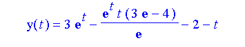
As you may have guessed, it gets a little more difficult to write the second derivative; D(D(y))(t) reprsents the derivative applied twice. If you wanted to represent the nth derivative, you could use the notation
(D@@n)(y)(t).A plot of the result is:
[> plot( rhs(%), t = 0..1 );
[> ?dsolve
Differentiation
We've covered so many advanced mathematical topics that it may be worth seeing that Maple can also do simple math. The differentiation command diff takes two arguments, the first is the expression to be differentated, the second is the variable of differentiation:
[> diff( sin(x)*x^2, x );
If you want to take a second derivative, just add another x:
[> diff( sin(x)*x^2, x, x );
Notice that the sine command looked at its argument, determined that it was unable to evaluate it into something useful (like a floating-point number) and therefore it left it as is.
[> ?diff
Integration
Integration may be done using the integration command int. Like the differentiation command, it takes a second argument, the variable of integration:
[> int( sin(x)*x^2, x );
Note that it does not add +c. You can also integrate over a range:
[> int( sin(x)*x^2, x );
Maple is also aware of indefinite integrals:
[> int( sin(x)/x, x = 0..infinity );
[> ?diff
Expand
The next function is the expand command. Given an expression, for example, a polynomial, the expand command will return an expanded polynomial. The command is also aware of various trigonometric relationships. For example:
[> expand( (x - 1)^2 * (x + 2)^3 + 2 );
[> expand( sin(a + b) );
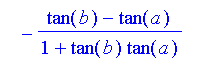
[> expand( tan(a - b) );
[> ?expand
Partial-Fraction Decomposition
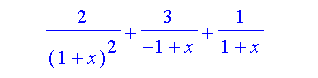
To find the partial-fraction decomposition of the rational polynomial 4(x2 + 2x)/(x3 + x2 − x − 1), we can use the convert command. This command takes a second argument which specifies the type of conversion (in this case parfrac) followed by the variable with which the decomposition should take place. For example,
[> convert( 4*(x^2 + 8*x)/(x^3 + x^2 - x - 1), parfrac, x );
[> ?convert,parfrac
Laplace Transforms
The last topic we will look at are Laplace transforms. For this, we must load the inttrans (integral transformations) package:
[> with( inttrans );
As you can see, there are other integral transformations, as well, including Fourier transforms.
The arguments of the laplace command are: the expression, the original variable, and the transformation variable. For example,
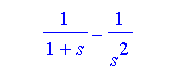
[> laplace( exp(-t) - t, t, s );
The command is also aware of other rules:
[> laplace( D(y)(t), t, s );
This is the familiar rule L(y(1))(t) = s L(y)(t) − y(0).
To find the inverse Laplace transform, use the invlaplace command with the two variables switched.
[> ?laplace
Plotting Functions of 1 and 2 Variables
Plotting on one dimension done through an adaptive algorithm which adds extra points were necessary to satisfy a heuristic smoothness.
[> plot( cos(3.23*x)*exp(-0.323*x), x = 0..20 );
Multiple functions can be plotted at once by providing a list of functions:
[> plot( [2.3*cos(3.23*x)*exp(-0.323*x), 2.3*sin(3.23*x)*exp(-0.323*x)],
   x = 0..20, y = -1..1, color=[red, blue] );
Plotting a function of two variables uses the plot3d procedure:
[> plot3d( x/sqrt(x^2 + y^2), x = -1..1, y = -1..1, axes = framed );
Plotting functions of two variables does not use adaptive plotting: if you want more detail, you must sample more points with the grid=[n, n] option.
[> plot3d( x/sqrt(x^2 + y^2), x = -1..1, y = -1..1,
   axes = framed, grid = [101, 101] );
[> ?plot
[> ?plot3d
Summary
Hopefully this has given you a nice introduction to some of the more interesting features of Maple as they may be needed by an engineering student. I have not gotten into the programming language features of Maple, as most likely, if you're going to do programming like that, it will be in C++ or Matlab. This page mostly covers those features which are unavailable in C++ or Matlab.
If you want, you can always visit the home page of Maplesoft, Inc.

Department of Electrical and Computer Engineering
University of Waterloo
200 University Avenue West
Waterloo, Ontario, Canada N2L 3G1
Website maintained by Douglas Wilhelm Harder