Not all data may be represented by functions in the form y = c1f1(x) + ... + cnfn(x), for example, many responses are exponential in nature, that is the data follows a curve of the form y = c1ec2x which is not in the desired form for linear regression.
We want to be able to transform the exponential function into a linear sum of functions. Here we will look at some transformations which may be used to convert such data so that we may use the least squares method to find the best fitting curve.
Note: Matlab uses the log function to calculate the natural logarithm, and therefore in these notes, we will use log(x) to calculate what you would normally write as ln(x) in your calculus course.
Theory
Assumptions
Suppose we have collected a number of data points which are known to follow an exponential curve of the form y = a eb x. That the data is exponential must be derived from the model or by observation.
Derivation
Given such data, if we take the natural logarithm of both sides of the equation y = a eb x, we get log(y) = log(a eb x) = log(a) + log(eb x) = log(a) + b x.
If we represent φ = log(y) and α = log(a), then this equation φ = α + b x, which is of the appropriate form for using least squares.
Using least squares, once we find α, we may set a = eα and therefore we have the coefficients a and b which describe the exponential curve which most closely passes through the given data points (xi, yi) for i = 1, 2, ..., n.
HOWTO
Problem
Given data (xi, yi), for i = 1, 2, ..., n which is known to approximate an exponential curve, find the best fitting exponential function of the form y(x) = aebx.
Assumptions
We will assume the model is correct and that the data is defined by two vectors x = (xi) and y = (yi).
Tools
We will use algebra and linear regression.
Process
Take the logarithm of the y values and define the vector φ = (φi) = (log(yi)).
Now, find the least-squares curve of the form c1 x + c2 which best fits the data points (xi, φi). See the Topic 6.1 Linear Regression.
Having found the coefficient vector c, the best fitting curve is
Examples
Example 1
Figure 1 shows data which comes from an exponentially decaying function.
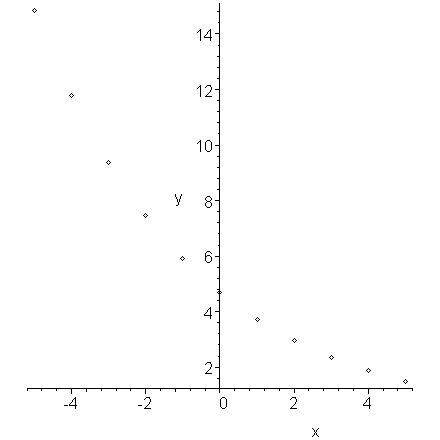
Figure 1. Exponentially decaying data.
If, for each x, we plot the logarithm of its associated y value, we get the plot in Figure 2 which is clearly linear.
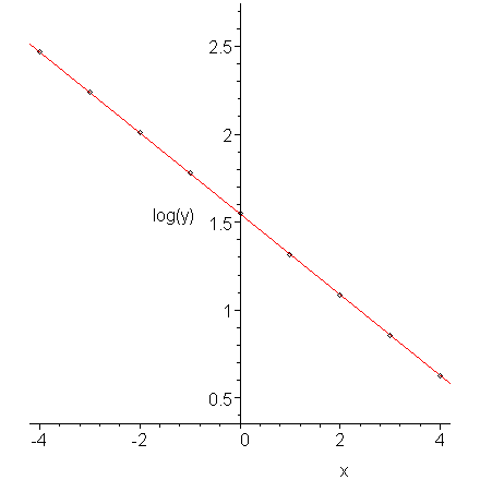
Figure 2. The logarithm of exponentially decaying data.
The data in Figure 1 comes from the function y = 4.7e-0.23x. The slope of the line (-0.23) in Figure 2 equals the rate of decay.
Example 2
Figure 3 shows data which is growing as a power of x, that is, y(x) = axb. Note that it must pass through the origin.
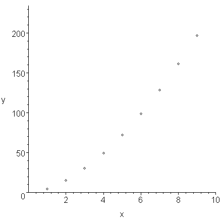
Figure 3. Data displaying power growth.
If we plot the logarithms of the x values versus the logarithms of the y values, we find that the points lie on a straight line.
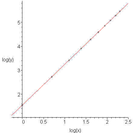
Figure 4. The log-log plot of data which displays power growth.
The data in Figure 3 comes from the function y = 4.7x1.7. The slope of the line (1.7) in Figure 4 equals the power.
Comment: you may hypothesize that the data in Figure 3 appears to be quadratic. We could try fitting a quadratic curve to this data, as is shown in Figure 5, however, we note that it is not as good a fit as the form which we found.
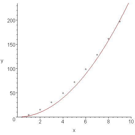
Figure 5. A fit of a least-squares quadratic curve y = 2.472x2 to the data in Figure 3.
Example 3
The following data is known to come from a discharging capacitor together with a loop containing a resistor. We are sampling periodically, that is, once every second.
(5, 0.05336), (6, 0.03179), (7, 0.01889), (8, 0.01123), (9, 0.00666),
(10, 0.00396)
This data is shown in Figure 6.
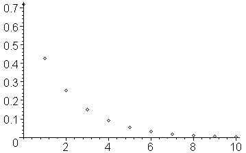
Figure 6. The given data points.
Taking the natural logarithm (the log function in Matlab) of each of the y values, we get the data:
(5, -2.93069), (6, -3.44852), (7, -3.96897), (8, -4.48958), (9, -5.01201),
(10, -5.53148)
Let us denote the logarithm of each of the y values by the vector φ = (-0.33315, -0.85352, ..., -5.53148)T.
If you plot this data, you will note that it does appear to be approximately linear and decreasing. This is shown in Figure 7.
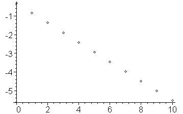
Figure 7. The given data points.
Thus, we should be able to fit a curve of the form c1x + c2 to the data. We may now define the general Vandermonde matrix
and therefore, solving VTVc = VTφ, for the coefficient vector c we get:
c = (-0.51986, -0.33131)T
and therefore, the best fitting line through the logarithmic data is -0.51986x - 0.33131, as can be seen in Figure 8.
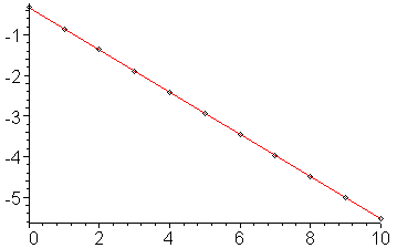
Figure 8. The least squares line which passes through the logarithms of the y values.
Therefore the best fitting line through the original is e-0.51986x - 0.33131 = e-0.51986xe- 0.33131 = 0.71798 e-0.51986x. The original data and this curve are shown in Figure 9.
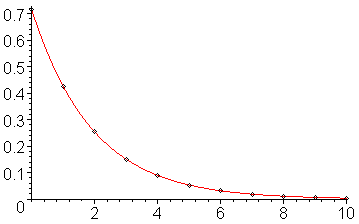
Figure 9. The least squares line which passes through the logarithms of the y values.
Note that while the line appears to go exactly through the points, if you explicitly calculate the y values on the line, you will see that they are only approximately equal (in this case, to about two decimal digits).
Engineering
The response of any linear system may be shown to have exponential responses when a system has zero input. For example, the charge on a capacitor decreases exponentially when placed in a loop together with a resistor.
It is possible to estimate the rate at which a capacitor is discharging by sampling the voltage across the capacitor periodically, and since it is known that the capacitor discharges exponentially, it would make more sense to try to fit the data points to an exponential function than it would be to try to use polynomial interpolation.
Power Transformation
Asymptotic run times may be determined with power transformations: data which is believed to run in Θ(nk) can be tested by finding the best-fitting line which passes through the points (ln(x1), ln(y1)), ..., (ln(xn), ln(yn)) and the slope of that line will approximate k.
This works whether n → ∞ (for example, an algorithm designed to work with a problem of size n) or n → 0 (for example, a numerical methods algorithm). We will use the power transformation to show that future methods converge as claimed.
Error
To be done later, though one comment: when we convert exponential data to linear data, because we are taking the logarithm of each of the y values, the resulting curve minimizes the sum of the squares of the logarithms of the errors, not the sum of the squares of the errors themselves, so the fit will be much more tight for smaller values.
Questions
Question 1
Find the least squares curve which fits the exponential data:
x = (0.029, 0.098, 0.213, 0.352, 0.376, 0.393, 0.473, 0.639, 0.855, 0.909)T
y = (2.313, 2.235, 2.094, 1.949, 1.924, 1.907, 1.828, 1.674, 1.493, 1.451)T
Answer: y = 2.3492e-0.53033x.
Question 2.
Find the least squares curve which fits the exponential data:
x = (0.228, 0.266, 0.268, 0.345, 0.351, 0.543, 0.667, 0.942, 0.959, 0.991)T
y = (0.239, 0.196, 0.218, 0.173, 0.188, 0.090, 0.057, 0.022, 0.026, 0.019)T
Answer: y = 0.52118 e-3.27260 x.
Matlab
Finding the coefficient vector in Matlab is very simple:
x = [0.53, 0.75, 1.22, 2.11, 3.25]';
y = [0.78, 0.81, 0.97, 1.28, 1.82]';
V = [x, ones(size(x))];
c = V \ log(y);
To plot the points and the best fitting curve, you can enter:
xs = (0:0.1:4)';
plot( x, y )
hold on
plot( xs, exp(c(1)*xs + c(2)) );
Be sure to issue the command hold off if you want to start with a clean plot window.
Maple
The following commands in Maple:
with(CurveFitting):
pts := [[0.53, 0.78], [0.75, 0.81], [1.22, 0.97], [2.11, 1.28], [3.25, 1.82]];
logpts := map( t -> [t[1], ln(t[2])], pts );
fn := LeastSquares( logpts, x, curve = a*x + b );
plots[pointplot]( pts );
plots[display]( plot( exp( fn ), x = 0..4 ), plots[pointplot]( pts ) );
calculates the least-squares line of best fit for given data points, a plot those points, and a plot of the points together with the best-fitting curve. This last plot is shown in Figure 1.
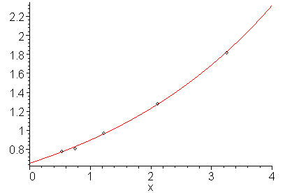
Figure 1. The given points and the least squares line passing through those points.
For more help on the least squares function or on the CurveFitting package, enter:
?CurveFitting,LeastSquares
?CurveFitting
Copyright ©2005 by Douglas Wilhelm Harder. All rights reserved.


