

The following commands in Maple:
with(CurveFitting):
pts := [[0.53, 0.78], [0.75, 0.81], [1.22, 0.97], [2.11, 1.28], [3.25, 1.82]];
logpts := map( t -> [t[1], ln(t[2])], pts );
fn := LeastSquares( logpts, x, curve = a*x + b );
plots[pointplot]( pts );
plots[display]( plot( exp( fn ), x = 0..4 ), plots[pointplot]( pts ) );
calculates the least-squares line of best fit for given data points, a plot those points, and a plot of the points together with the best-fitting curve. This last plot is shown in Figure 1.
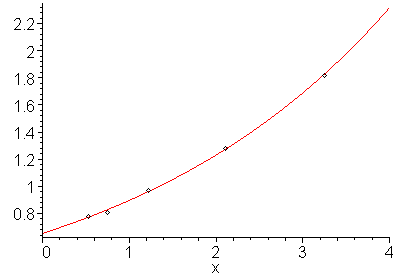
Figure 1. The given points and the least squares line passing through those points.
For more help on the least squares function or on the CurveFitting package, enter:
?CurveFitting,LeastSquares
?CurveFitting
Copyright ©2005 by Douglas Wilhelm Harder. All rights reserved.
