Newton's method is a technique for finding the root of a scalar-valued function f(x) of a single variable x. It has rapid convergence properties but requires that model information providing the derivative exists.
Background
Useful background for this topic includes:
- 3. Iteration
- 7. Taylor series
- 10.3 Newont's method
References
- Stoer, Section 5.1, The Development of Iterative Methods, p.263.
Theory
Assumptions
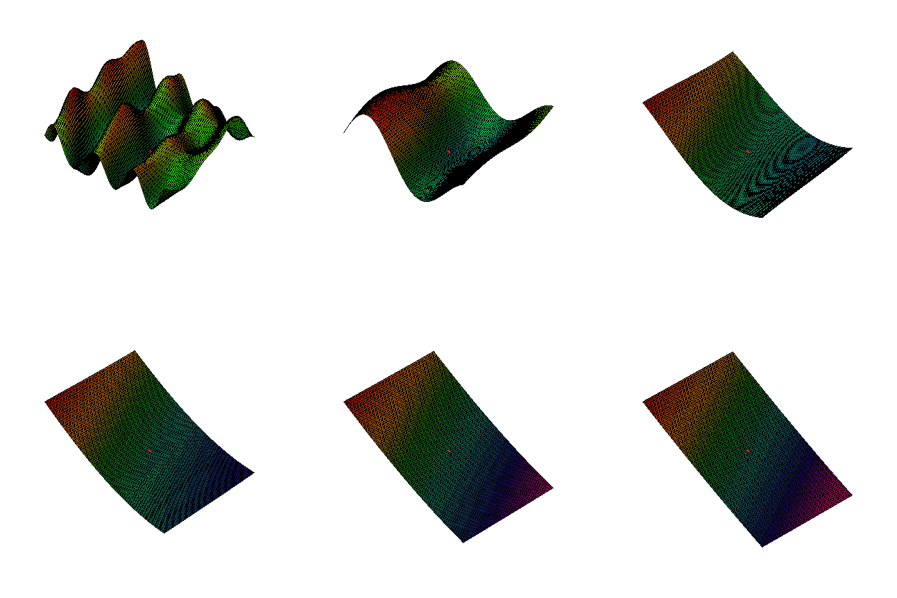
This method is based on the assumption that any function with continuous partial derivatives looks like an n dimensional plane. For example, Figure 1 zooms in on a two-dimensional function with continuous partial derivatives. While the function looks reasonably wild, as you zoom in on the red dot, the function looks more and more like a flat plane.

Figure 1. Zoom on a function of two variables.
Similar to Newton's method in one dimension, we will assume that each of the n functions which make up f(x) have continuous partial derivatives which we can compute.
Partial Derivation
To be filled later.
HOWTO
Problem
Given n functions, each of n variables (given by a vector x), fi(x), find a vector r (called a root) such that f(r) = 0.
We will write the n functions as a vector-valued function f(x).
Assumptions
We will assume that each of the functions fi(x) is continuous and has continuous partial derivatives.
Tools
We will use sampling, partial derivatives, iteration, and solving systems of linear equations. Information about the partial derivatives is derived from the model.
Initial Requirements
We have an initial approximation x0 of the root.
We have calculated the Jacobian J(f)(x).
Iteration Process
Given the approximation xn, we solve the system of linear equations defined by
J(f)(xn) Δxn = -f(xn)
for Δxn and then set:
xn + 1 = xn + Δxn
Halting Conditions
There are three conditions which may cause the iteration process to halt (where the norm used may be any of the 1, 2, or infinity norms):
- We halt if both of the following conditions are met:
- The step between successive iterates is sufficiently small, ||xn + 1 - xn|| < εstep, and
- The function evaluated at the point xn + 1 is sufficiently small, ||f(xn + 1)|| < εabs.
- If the Jacobian is indeterminate, that is, the determinant |J(f)(xn)| = 0, the iteration process fails and we halt.
- If we have iterated some maximum number of times, say N, and have not met Condition 1, we halt and indicate that a solution was not found.
If we halt due to Condition 1, we state that xn + 1 is our approximation to the root.
If we halt due to either Condition 2 or 3, we may either choose a different initial approximation x0, or state that a solution may not exist.
Examples
Example 1
A Maple worksheet showing Newton's method in 2 dimensions is given here. If Maple does not automatically open, save this file on your desktop, start Maple, and open the file. If you want to view this worksheet in HTML, click here.
Note: if you download the worksheet and run Maple, you will be able to select the images and rotate them. This would help in seeing the points and understanding how the approximations converge. Maple is available on all Engineering computers.
Example 2
Approximate a root of the function f(x) defined by:
Let our initial approximation be x0 = (0, 0)T.
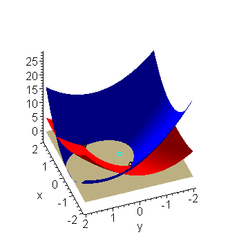
To visualize this, we have two functions (the first red, the second blue), each of two variables, defining two surfaces. We want to find a point where both functions are simultaneously zero. Thus, we are looking for either of the two black points in Figure 1 (click to enlarge the image). The two roots are (0.849308816, 0.9927594664)T and (-0.6397934171, -0.1918694996)T

Figure 1. The two functions in Example 1, the roots (black) and our initial approximation (0, 0)T (cyan).
Next, we calculate the Jacobian:
The first column is f(x) with partial derivatives with respect to x, and the second column is f(x) with partial derivatives with respect to y. We will continue iterating until ||Δxn||1 < εstep = 0.01 and ||f(xn + 1||1 < εabs = 0.01. Recall that the 1 norm of a vector is the sum of the absolute values of the entries.
Rather than tabulating the results, we will explicitly compute each iteration:
Calculating x1
Evaluating both the Jacobian J(f)(x0) and -f(x0), we get the system:
Solving this for Δx0, we get Δx0 = (-1.0, -0.66667)T, and therefore our next approximation is:
We note that, using the 1 norm, ||Δx0||1 = 1.6667 and ||f(x1)||1 = 5.7778.
Calculating x2
Evaluating both the Jacobian J(f)(x1) and -f(x1), we get the system:
Solving this for Δx1, we get Δx1 = (0.12483, 0.55851)T, and therefore our next approximation is:
We note that, using the 1 norm, ||Δx1||1 = 0.68334 and ||f(x2)||1 = 1.3102.
Calculating x3
Evaluating both the Jacobian J(f)(x2) and -f(x2), we get the system:
Solving this for Δx2, we get Δx2 = (0.20229, -0.079792)T, and therefore our next approximation is:
We note that, using the 1 norm, ||Δx2||1 = 0.28208 and ||f(x3)||1 = 0.1892.
Calculating x4
Evaluating both the Jacobian J(f)(x3) and -f(x3), we get the system:
Solving this for Δx3, we get Δx3 = (0.032496, -0.0040448)T, and therefore our next approximation is:
We note that, using the 1 norm, ||Δx3||1 = 0.036541 and ||f(x4)||1 = 0.0042.
Calculating x5
Evaluating both the Jacobian J(f)(x4) and -f(x4), we get the system:
Solving this for Δx4, we get Δx4 = (0.00056451, 0.00016391)T, and therefore our next approximation is:
We note that, using the 1 norm, ||Δx4||1 = 0.0042 and ||f(x5)||1 = 0.0001.
Final Solution
We may therefore stop and we use x5 = (-0.63982, -0.19183)T as our approximation to the root. The actual root is (-0.6397934171, -0.1918694996)T, and thus we have a reasonable approximation.
To find the other root, we would have to choose a different initial point x0.
Engineering
No applications yet.
Error
The error analysis is beyond the scope of this course, but is similar to that of Newton's method in one dimension, that is, it is O(h2) where h is the magnitude of the error of our current approximation.
Questions
Question 1
Perform three iterations to approximate a root of the system described by
starting with the point x0 = (1, 1)T.
Answer: x1 = (0.6666667, 1.833333)T, x2 = (0.5833333, 1.643939)T and x3 = (0.5773810, 1.633030)T. Incidentally, this is closest to the root (0.5773502693, 1.632993162)T (there are four altogether).
Question 2
What happens if you start with x0 = (0, 0)T in Question 1?
Question 3
Perform three iterations to approximate a root of the system described by
starting with the point x0 = (-1.5, 0.5)T.
Answer: x1 = (-1.375, 0.575)T, x2 = (-1.36921, 0.577912)T and x3 = (-1.36921, 0.577918)T. Incidentally, this is closest to the root (-1.369205407, 0.577917560)T (there are four altogether).
Question 4
From the symmetry in the function given in Question 3, can you guess another root?
Answer: By symmetry, (0.577918, -1.36921)T would approximate another root because if you swap all xs and ys in the function you get the same expression.
Matlab
To be filled later.
Maple
You can download this Maple worksheet to visualize Newton's method in two dimensions. Save this file as newton2d.mws and open it with whichever version of Maple running on your machine (probably Maple 9).
Copyright ©2005 by Douglas Wilhelm Harder. All rights reserved.


