Example 1
A Maple worksheet showing Newton's method in 2 dimensions is given here. If Maple does not automatically open, save this file on your desktop, start Maple, and open the file. If you want to view this worksheet in HTML, click here.
Note: if you download the worksheet and run Maple, you will be able to select the images and rotate them. This would help in seeing the points and understanding how the approximations converge. Maple is available on all Engineering computers.
Example 2
Approximate a root of the function f(x) defined by:
Let our initial approximation be x0 = (0, 0)T.
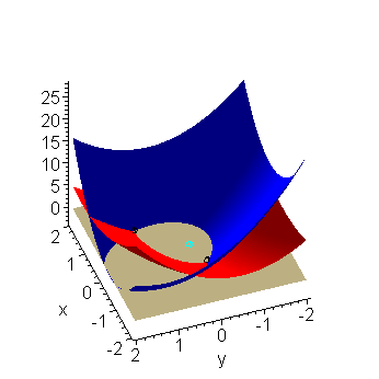
To visualize this, we have two functions (the first red, the second blue), each of two variables, defining two surfaces. We want to find a point where both functions are simultaneously zero. Thus, we are looking for either of the two black points in Figure 1 (click to enlarge the image). The two roots are (0.849308816, 0.9927594664)T and (-0.6397934171, -0.1918694996)T

Figure 1. The two functions in Example 1, the roots (black) and our initial approximation (0, 0)T (cyan).
Next, we calculate the Jacobian:
The first column is f(x) with partial derivatives with respect to x, and the second column is f(x) with partial derivatives with respect to y. We will continue iterating until ||Δxn||1 < εstep = 0.01 and ||f(xn + 1||1 < εabs = 0.01. Recall that the 1 norm of a vector is the sum of the absolute values of the entries.
Rather than tabulating the results, we will explicitly compute each iteration:
Calculating x1
Evaluating both the Jacobian J(f)(x0) and -f(x0), we get the system:
Solving this for Δx0, we get Δx0 = (-1.0, -0.66667)T, and therefore our next approximation is:
We note that, using the 1 norm, ||Δx0||1 = 1.6667 and ||f(x1)||1 = 5.7778.
Calculating x2
Evaluating both the Jacobian J(f)(x1) and -f(x1), we get the system:
Solving this for Δx1, we get Δx1 = (0.12483, 0.55851)T, and therefore our next approximation is:
We note that, using the 1 norm, ||Δx1||1 = 0.68334 and ||f(x2)||1 = 1.3102.
Calculating x3
Evaluating both the Jacobian J(f)(x2) and -f(x2), we get the system:
Solving this for Δx2, we get Δx2 = (0.20229, -0.079792)T, and therefore our next approximation is:
We note that, using the 1 norm, ||Δx2||1 = 0.28208 and ||f(x3)||1 = 0.1892.
Calculating x4
Evaluating both the Jacobian J(f)(x3) and -f(x3), we get the system:
Solving this for Δx3, we get Δx3 = (0.032496, -0.0040448)T, and therefore our next approximation is:
We note that, using the 1 norm, ||Δx3||1 = 0.036541 and ||f(x4)||1 = 0.0042.
Calculating x5
Evaluating both the Jacobian J(f)(x4) and -f(x4), we get the system:
Solving this for Δx4, we get Δx4 = (0.00056451, 0.00016391)T, and therefore our next approximation is:
We note that, using the 1 norm, ||Δx4||1 = 0.0042 and ||f(x5)||1 = 0.0001.
Final Solution
We may therefore stop and we use x5 = (-0.63982, -0.19183)T as our approximation to the root. The actual root is (-0.6397934171, -0.1918694996)T, and thus we have a reasonable approximation.
To find the other root, we would have to choose a different initial point x0.
Copyright ©2005 by Douglas Wilhelm Harder. All rights reserved.


