

Romberg integration is an extrapolation technique which allows us to take a sequence approximate solutions to an integral and calculate a better approximation. This technique assumes that the function we are integrating is sufficiently differentiable.
Background
Useful background for this topic includes:
References
- Bradie, 6.7 Romberg Integration, p.496
- Mathews, 7.3 Recursive Rules and Romberg Integration, p.378
- Weisstein, http://mathworld.wolfram.com/RombergIntegration.html.
Theory
Assumptions
We will assume that f(x) is a scalar-valued function of a single variable x and that f(x) is sufficiently differentiable.
Derivation
We know from the composite-trapezoidal rule that the error for approximating the integral is approximately
Let I represent the actual value of the integral:
Therefore, let E0,0 and E1,0 be the errors for approximating the integral with 1 and 2 interval, respectively:
I = R1,0 + E1,0
Graphically, this may be visualized in Figure 1 which shows these two errors. The point on the left is the actual value.
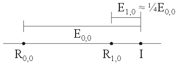
Figure 1. The errors E0,0 and E1,0.
If the error is reduced approximately by ¼ with each iteration, then E1,0 ≈ ¼ E0,0.
Looking at Figure 1, we note that if E1, 0 = ¼E0, 0, then R1, 0 − R0, 0 = ¾ E0, 0. Therefore, we have that
Therefore, we can solve for E0, 0 to get that
We can simplify this to get the approximation:
We will denote this approximation with R1,1.
To show that this really works, let us consider integrating the function f(x) = e-x on the interval [0, 2]. The actual answer is 0.8646647168.
If we approximate the integral with the composite-trapezoidal rule using 1, 2, and 4 intervals, we get the three approximations:
R1, 0 = ½(e-0 + 2e-1 + e-2)⋅1 ≈ 0.9355470828
R2, 0 = ½(e-0 + 2e-0.5 + 2e-1 + 2e-1.5 + e-2)⋅0.5 ≈ 0.9355470828
We see the error is going down, however, if we use our formula, we get:
R2, 1 = (4 R2,0 − R1,0)/3 ≈ 0.8649562404
The absolute errors are 0.00429 and 0.000292.
At this point, you may ask whether or not it is worth repeating the same process, but now with R1, 1 and R2, 1. Unfortunately, if we try this, we note that the error increases: the absolute error of (4 R2,1 − R1,1)/3 is 0.00104, which is worse than the error for R2, 1.
However, there is another fact we may note: If we consider the ratio of the error of R1, 1 over the error of R2, 1, we get 0.00429/0.000292 = 14.69. Previously, the error dropped by a factor of 4, here, it may not be unreasonable to postulate that the error is dropping by a factor of 42 = 16, however, we should show this.
To prove this fact, we must look at Taylor series:
If we represent the integral by I, then suppose that T(h) is an approximation of I using intervals of width h. In this case, a small change in:
HOWTO
Problem
Given a function of one variable, f(x), find the integral on the interval
Assumptions
We will assume that the function f(x) is sufficiently differentiable.
Tools
We will use sampling, iteration, and the composite-trapezoidal rule. Let Tn be the approximation of the above integral using the composite-trapezoidal rule with 2n subintervals.
Initial Requirements
Let R0, 0 = T0.
Iteration Process
Having calculated Rn, 0, Rn, 1, ..., Rn, n, proceed as follows:
Set Rn + 1, 0 = Tn + 1.
Next, for j = 1, ..., n + 1, calculate
For example, Figure 1 shows the order (the circled red numbers) in which the entries Ri, j are calculated. The numbers in the first column are calculated using the composite-trapezoidal rule. For the other entries, the numbers on the arrows indicate the coefficients of the weighted average used to create that entry. This denominator of the weighted average is the sum of the two numbers.
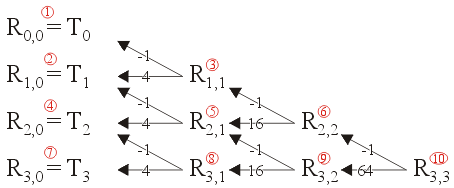
Figure 1. Calculating the Romberg approximations.
Halting Conditions
There are two conditions which may cause the iteration process to halt:
- We halt if the step between successive iterates is sufficiently small, that is, |Rn + 1, n + 1 - Rn, n| < εstep, and
- If we have iterated some maximum number of times, say N, and have not met Condition 1, we halt and indicate that a solution was not found.
If we halt due to Condition 1, we state that Rn + 1, n + 1 is our approximation to the integral.
If we halt due to Condition 2, we state that a solution may not exist.
Examples
Example 1
Integrate the function sin(x) on the interval [a, b] = [0, &pi]. From calculus, you know that the answer is 2. Continue iterating until εstep < 1e-5.
Let h = b - a = π. Then
R0, 0 = T(h) = ½(sin(0) + sin(π))π = 0
Now, for i = 1, 2, ..., we calculate:
i = 1
R1,0 = T(π/2) = 1.5707963267948966192
- (4 ⋅ 1.5707963267948966192 - 0)/3 = 2.0943951023931954923
i = 2
R2,0 = T(π/4) = 1.8961188979370399
- (4 ⋅ 1.8961188979370399 - 1.5707963267948966)/3 = 2.0045597549844210
- (16 ⋅ 2.0045597549844210 - 2.0943951023931955)/15 = 1.9985707318238360
i = 3
R3,0 = T(π/8) = 1.9742316019455508
- (4 ⋅ 1.9742316019455508 - 1.8961188979370399)/3 = 2.0002691699483878
- (16 ⋅ 2.0002691699483878 - 2.0045597549844210)/15 = 1.9999831309459856
- (64 ⋅ 1.9999831309459856 - 1.9985707318238360)/63 = 2.0000055499796705
i = 4
R4,0 = T(π/16) = 1.9935703437723393
- (4 ⋅ 1.9935703437723393 - 1.9742316019455508)/3 = 2.0000165910479355
- (16 ⋅ 2.0000165910479355 - 2.0002691699483878)/15 = 1.9999997524545720
- (64 ⋅ 1.9999997524545720 - 1.9999831309459856)/63 = 2.0000000162880417
- (256⋅2.0000000162880417 - 2.0000055499796705)/255 = 1.9999999945872902
Finally, |1.9999999945872902 - 2.0000055499796705| ≈ 0.00000556, and thus we may halt and our approximation of the integral is 1.9999999945872902 .
Engineering
No applications yet.
Error
Assuming the function is sufficiently differentiable, the error of Rn, n is O(h2n + 2) (that is, it will be some multiple of h2n + 2).
Questions
Question 1
Use Romberg integration to approximate the integral of f(x) = cos(x) on the interval [0, 3] and iterate until εstep < 1e-5 or N = 10. Begin with an interval width of with h = 3.
Answer: 0.141120007827708
Question 2
Use Romberg integration to approximate the integral of f(x) = x5 on the interval [0, 4].
Answer: 682.666666666667 (you should have gotten a zero difference at the last step)
Matlab
Approximate the integral of f(x) = cos(x) until εstep < 1e-10 or N = 10.
Please note, because we cannot begin at R(0, 0), each index will be off by one. This is not optimal code, either.
format long
eps_step = 1e-10;
N = 10;
R = zeros( N + 1, N + 1 );
a = 0;
b = 10;
h = b - a;
R(0 + 1, 0 + 1) = 0.5*(cos(a) + cos(b))*h;

for i = 1:N
    h = h/2;
    % This calculates the trapezoidal rule with intervals of width h
    R( i + 1, 1 ) = 0.5*(cos(a) + 2*sum( cos( (a + h):h:(b - h) ) ) + cos(b))*h;

    for j = 1:i
        R(i + 1, j + 1) = (4^j*R(i + 1, j) - R(i, j))/(4^j - 1);
    end

    if abs( R(i + 1, i + 1) - R(i, i) ) < eps_step
       break;
    elseif i == N + 1
       error( 'Romberg integration did not converge' );
    end
end

R( i + 1, i + 1 )
The correct answer to 20 decimal digits is sin(10) = -0.54402111088936981340.
Maple
The following commands in Maple:
with( Student[Calculus1] ):
R := Array( 0..5, 0..5, 0 ):
R[0,0] := Student:-Calculus1:-ApproximateInt( exp(-x)*cos(x), x = 0.0..10.0,
   method = trapezoid, partition = 1 ):

for i from 1 to 5 do
   R[i, 0] := Student:-Calculus1:-ApproximateInt( exp(-x)*cos(x), x = 0.0..10.0,
      method = trapezoid, partition = 2^i );
   for j from 1 to i do
      R[i, j] := (4^j*R[i, j - 1] - R[i - 1, j - 1])/(4^j - 1);
   end do;
end do:

convert( R, Matrix );
int( exp(-x)*cos(x), x = 0..10 );
evalf( % );
For more help on ApproximateInt or on the Student[Calculus1] package, enter:
?ApproximateInt
?Student,Calculus1
Copyright ©2005 by Douglas Wilhelm Harder. All rights reserved.
