Introduction Notes Theory HOWTO Examples Engineering Error Questions Matlab Maple

Assumptions

We will assume that f(x) is a scalar-valued function of a single variable x and that f(x) is sufficiently differentiable.

Derivation

We know from the composite-trapezoidal rule that the error for approximating the integral is approximately

Let I represent the actual value of the integral:

Therefore, let E_0,0 and E_1,0 be the errors for approximating the integral with 1 and 2 interval, respectively:

I = R_0,0 + E_0,0
I = R_1,0 + E_1,0

Graphically, this may be visualized in Figure 1 which shows these two errors. The point on the left is the actual value.

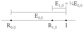
Figure 1. The errors E_0,0 and E_1,0.

If the error is reduced approximately by ¼ with each iteration, then E_1,0 ≈ ¼ E_0,0.

Looking at Figure 1, we note that if E_{1, 0} = ¼E_{0, 0}, then R_{1, 0} − R_{0, 0} = ¾ E_{0, 0}. Therefore, we have that

R_{1, 0} − R_0,0 ≈ ¾E_{0, 0}

Therefore, we can solve for E_{0, 0} to get that

We can simplify this to get the approximation:

We will denote this approximation with R_1,1.

To show that this really works, let us consider integrating the function f(x) = e^-x on the interval [0, 2]. The actual answer is 0.8646647168.

If we approximate the integral with the composite-trapezoidal rule using 1, 2, and 4 intervals, we get the three approximations:

R_{0, 0} = ½(e^-0 + e^-2)⋅2 ≈ 1.135335283
R_{1, 0} = ½(e^-0 + 2e^-1 + e^-2)⋅1 ≈ 0.9355470828
R_{2, 0} = ½(e^-0 + 2e^-0.5 + 2e^-1 + 2e^-1.5 + e^-2)⋅0.5 ≈ 0.9355470828

We see the error is going down, however, if we use our formula, we get:

R_{1, 1} = (4 R_1,0 − R_0,0)/3 ≈ 0.8689510160
R_{2, 1} = (4 R_2,0 − R_1,0)/3 ≈ 0.8649562404

The absolute errors are 0.00429 and 0.000292.

At this point, you may ask whether or not it is worth repeating the same process, but now with R_{1, 1} and R_{2, 1}. Unfortunately, if we try this, we note that the error increases: the absolute error of (4 R_2,1 − R_1,1)/3 is 0.00104, which is worse than the error for R_{2, 1}.

However, there is another fact we may note: If we consider the ratio of the error of R_{1, 1} over the error of R_{2, 1}, we get 0.00429/0.000292 = 14.69. Previously, the error dropped by a factor of 4, here, it may not be unreasonable to postulate that the error is dropping by a factor of 4² = 16, however, we should show this.

To prove this fact, we must look at Taylor series:

If we represent the integral by I, then suppose that T(h) is an approximation of I using intervals of width h. In this case, a small change in:

T(h) = I + K₁h² + K₁h⁴ + K₁h⁶ + ⋅⋅⋅

Topic 13.3: Romberg Integration (Theory)

Assumptions

Derivation