By using a similar strategy to the trapezoidal rule to find a better approximation to an IVP in Heun's method, consider now Simpson's rule, where not only the end points, but also the interior points of the interval are sampled.
The 4th-order Runge Kutta method is similar to Simpson's rule: a sample of the slope is made at the mid-point on the interval, as well as the end points, and a weighted average is taken, placing more weight on the slope at the mid point.
It should be noted that Runge-Kutta refers to an entire class of IVP solvers, which includes Euler's method and Heun's method. We are looking at one particularly effective, yet simple, case.
Given the IVP
y(t0) = y0
if we want to estimate y(t1), we set h = t1 − t0. Remember that f( t, y ) gives the slope at the point (t, y). Thus, we can find the slope at (t0, y0):
Next, we use this slope to estimate y(t0 + h/2) ≈ y0 + ½ hK0 and sample the slope at this intermediate point:
Using this new slope, we estimate y(t0 + h/2) ≈ y0 + ½ hK1 and sample the slope at this new point:
Finally, we use this last approximation of the slope to estimate y(t1) = y(t0 + h) ≈ y0 + hK2 and sample the slope at this point:
All four of these slopes, K0, K1, K2, and K3 approximate the slope of the solution on the interval [t0, t1], and therefore we take the following weighted average:
Therefore, we approximate y(t1) by
Note how the two values K1 and K2 both approximate the slope at the midpoint. Thus, the averaging is very similar to Simpson's rule which also places a weight of 4 on the midpoint.
Graphical Representation
To view this graphically, let's consider the IVP
y(0) = 0.5
Figure 1 shows Euler's approximation of y(1), that is, following the slope K0 = f(t0, y0) = 1.25, we get that y(0.5) ≈ 0.5 + 0.5 ⋅ 1.25 = 1.125.
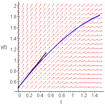
Figure 1. Euler's approximation to the value of y(0.5).
If we sample the slope at (0.5, 1.125), we find that it is K1 = f(0.5, 1.125) = 1.0625. This slope is shown as a light-blue line in Figure 2.
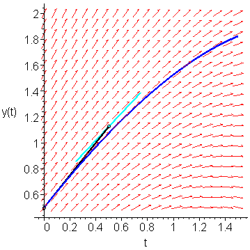
Figure 2. The slope at the point (0.5, 1.125).
We can use this second slope to approximate y(0.5) ≈ 0.5 + 0.5 ⋅ K1 = 1.03125. This is shown in Figure 3.
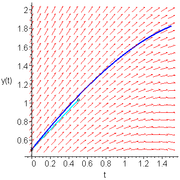
Figure 3. Following the slope K1 out a distance h/2 = 0.5.
If we sample the slope at (0.5, 1.03125), we find that it is K2 = f(0.5, 1.03125) = 1.015625. This slope is shown as a gold line in Figure 4.
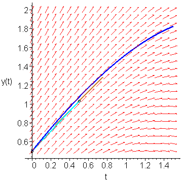
Figure 4. The slope at the point (0.5, 1.03125).
Finally, we can use this third slope to approximate y(1.0) ≈ 0.5 + 1 ⋅ K2 = 1.515625. This is shown in Figure 5.
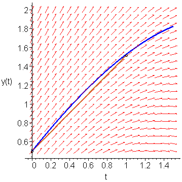
Figure 5. Following the slope K2 out a distance h = 1.
If we sample the slope at (1, 1.515625), we find that it is K3 = f(l, 1.515625) = 0.7578125. This slope is shown as a magenta line in Figure 4.
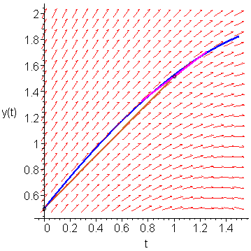
Figure 6. The slope at the point (1, 1.515625).
The weighted average of these four slopes is 1.02734375. Therefore, we approximate y(t1) by following this average slope out a distance 1: y1 = y0 + 1.02734375 ⋅ 1 = 1.527343750. This is shown in Figure 7. Note the significant improvement in the approximation as compared to that found by Heun's method.
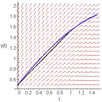
Figure 7. 4th-order Runge Kutta approximation to y(1).
Copyright ©2005 by Douglas Wilhelm Harder. All rights reserved.


