Introduction Notes Theory HOWTO Examples Engineering Error Questions Matlab Maple

We have worked with 1st-order initial-value problems. In this topic, we discuss how we can convert an nth-order initial-value problem (an nth-order differential equation and n initial values) into a system of n 1st-order initial-value problems.

Background

Useful background for this topic includes:

4. Linear Algebra
14.7 Higher-order Initial-value Problems

References

Bradie, Section 7.8, Systems of Equations and Higher-Order Equations, p.628.
Mathews, Section 9.7, Systems of Differential Equations, p.521.

Theory

To this point, we have considered IVPs with 1st-order

Consider an nth order IVP which consists of an nth order ODE and n initial conditions:

y⁽ⁿ⁾(t) = f( t, y(t), y⁽¹⁾(t), y⁽²⁾(t), ..., y^{(n − 1)}(t) )
y(t₀) = y₀
y⁽¹⁾(t₀) = y₀⁽¹⁾
y⁽²⁾(t₀) = y₀⁽²⁾
⋅
⋅
y^{(n − 1)}(t₀) = y₀^{(n − 1)}

For example,

y⁽²⁾(t) = 4 − sin(t) + y(t) − 2 y⁽¹⁾(t)
y(0) = 1
y⁽¹⁾(0) = 2

y⁽³⁾(t) = y(t) − t y⁽¹⁾(t) + 4 y⁽²⁾(t)
y(2) = 1
y⁽¹⁾(2) = 2
y⁽²⁾(2) = 3

Suppose we want to find the estimate y₁ of y(t₁). To do this we will convert the nth-order IVP into a system of n 1st-order IVPs by defining:

y₀(t) = y(t)
y₁(t) = y⁽¹⁾(t)
y₂(t) = y⁽²⁾(t)
⋅
⋅
y_{n − 1}(t) = y^{(n − 1)}(t)

We note that for i = 0, 1, ..., n − 2, the derivative y_i⁽¹⁾(t) = y_i + 1⁽¹⁾(t) and that y_n - 1⁽¹⁾(t) = f( t, y₀(t), y₁(t), y₂(t), ..., y_n − 1(t) ).

The initial conditions may now be converted to

y₀(t₀) = y₀
y₁(t₀) = y₀⁽¹⁾
y₂(t₀) = y₀⁽²⁾
⋅
⋅
y_{n − 1}(t₀) = y₀^{(n − 1)}

If we now define the vectors:

and

and the vector valued function:

then our initial value problem becomes the following vector-valued initial value problem:

y⁽¹⁾(t) = f( t, y(t) )
y(t₀) = y₀

where the derivative of the vector y(t) is the vector of element-wise derivatives.

Any of the techniques we have seen, Euler's method, Heun's method, 4th-order Runge Kutta, or the backward-Euler's method may be applied to approximate y(t₁).

Given our approximation y₁ = (y_{1, i}) of y(t₁), we find that y(t₁) ≈ y_{1, 1}. We also get, for free, approximations of y⁽¹⁾(t₁) ≈ y_{1, 2}, y⁽²⁾(t₁) ≈ y_{1, 3}, ..., and y^{(n − 1)}(t₁) ≈ y_{1, n}.

Additionally, we may apply any of the multiple-step methods, including Runge Kutta Fehlberg.

Example

If we look at the two problems shown above, we could rewrite the first:

y⁽²⁾(t) = 4 − sin(t) + y(t) − 2 y⁽¹⁾(t)
y(0) = 1
y⁽¹⁾(0) = 2

by defining

where the 2nd-order ODE may now be written as the following system of ODEs

with the initial condition

The second example,

y⁽³⁾(t) = y(t) − t y⁽¹⁾(t) + 4 y⁽²⁾(t)
y(2) = 1
y⁽¹⁾(2) = 2
y⁽²⁾(2) = 3

may be rewritten as a system of three functions:

where the 3rd-order ODE may now be written as the following system of ODEs

with the initial condition

We may now solve either of these systems of IVPs using the techniques explained in the previous topic on systems of IVPs.

HOWTO

Problem

Given the IVP

y⁽ⁿ⁾(t) = f( t, y(t), y⁽¹⁾(t), y⁽²⁾(t), ..., y^{(n − 1)}(t) )
y(t₀) = y₀
y⁽¹⁾(t₀) = y₀⁽¹⁾
y⁽²⁾(t₀) = y₀⁽²⁾
⋅
⋅
⋅
y^{(n − 1)}(t₀) = y₀^{(n − 1)}

approximate y(t₁).

Assumptions

The function f(t, y, y(t), y⁽¹⁾(t), y⁽²⁾(t), ..., y^{(n − 1)}(t)) should be continuous in all variables.

Tools

We will convert the nth-order IVP into a system of 1st-order IVPs and then use the techniques we have seen for IVPs.

Process

Define:

y₀(t) = y(t)
y₁(t) = y⁽¹⁾(t)
y₂(t) = y⁽²⁾(t)
⋅
⋅
y_{n − 1}(t) = y^{(n − 1)}(t)

and

y₀(t₀) = y₀
y₁(t₀) = y₀⁽¹⁾
y₂(t₀) = y₀⁽²⁾
⋅
⋅
y_{n − 1}(t₀) = y₀^{(n − 1)}

Next, define the vector-valued function

the vector-valued function

and the initial vector

we may now write the nth-order IVP as the 1st-order IVP

y⁽¹⁾(t) = f( t, y(t) )
y(t₀) = y₀

We may now use all the techniques we have used for 1st-order IVPs, only now, to vectors instead of scalars.

Examples

Example 1

Perform three approximations using Euler's method for the IVP

y⁽²⁾(t) = 4 − sin(t) + y(t) − 2 y⁽¹⁾(t)
y(0) = 1
y⁽¹⁾(0) = 2

with a step size of h = 0.1.

Using the rewritten derivative

we may calculate:

y₁ = y₀ + h f(0, y₀) = (1.2, 2.1)^T
y₂ = y₁ + h f(h, y₁) = (1.41, 2.1900166583)^T
y₃ = y₂ + h f(2h, y₂) = (1.62900166583, 2.2731463936)^T

Consequently, the approximation of the solution comprises the points

(0, 1), (0.1, 1.2), (0.2, 1.41), (0.3, 1.62900166583)

and the derivatives at these points are 2, 2.1, 2.1900166583, and 2.2731463936, respectively.

Example 2

Perform two approximations using Heun's method for the IVP

y⁽³⁾(t) = y(t) − t y⁽¹⁾(t) + 4 y⁽²⁾(t)
y(2) = 1
y⁽¹⁾(2) = 2
y⁽²⁾(2) = 3

with a step size of 0.1

In the theory section, we saw that this IVP can be converted into the system

and therefore, we may calculate:

K₀ = f( 0, y₀ ) = (2, 3, 13)^T
K₁ = f( h, y₀ + hK₀ ) = (2.3, 4.3, 18.17)^T

Therefore,

y₁ = y₀ + h (K₀ + K₀)/2 = (1.215, 2.365, 4.5585)^T

To approximate the next point, we repeat the process:

K₀ = f( h, y₁ ) = (2.365, 4.5585, 19.2125)^T
K₁ = f( 2h, y₁ + hK₀ ) = (2.82085, 6.47975, 26.80633)^T

Therefore,

y₂ = y₁ + h (K₀ + K₀)/2 = (1.4742925, 2.9169125, 6.8594415)^T

Consequently, the approximations to the solution are (0, 1), (0.1, 1.215), and (0.2, 1.4742925).

The derivatives at these three points are 2, 2.365, and 2.9169125, respectively, and the Nd derivatives at these points are 3, 4.5585, and 6.8594415, respectively.

Example 3

As an example of a stiff differential equation, you saw the Van der Pol 2nd-order ordinary differential equation:

y⁽²⁾(t) − μ(1 − y(t)²) y⁽¹⁾(t) + y(t) = 0

We can rewrite this in the desired form:

y⁽²⁾(t) = μ(1 − y(t)²) y⁽¹⁾(t) − y(t)

Let μ = 0.3 and let the initial conditions be y(0) = 0.7 and y⁽¹⁾(0) = 1.2 and therefore, we may convert this to the system:

and

with the initial conditions

For simplicity, we will explicitly solve this system using multiple steps of Euler's method. We deliberately choose a very small value of h = 0.1 to avoid the stiff properties of this ODE and we define t_i = ih. Thus, for i = 1, 2, ..., 1000, we will solve:

y_i = y_{i − 1} + h f( t_{i − 1}, y_{i − 1})

Therefore, for the first step, we have:

The next three iterations are

The term of primary interest is the first of each of the points. If we plot the points (t_i, y_{i, 1}), we get the oscillating curve in Figure 1.

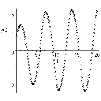
Figure 1. An approximation of the solution to our IVP.

Rather than plotting the points, we can connect the points with a line, as is shown in Figure 2.

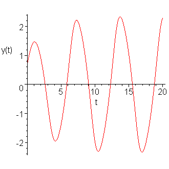
Figure 2. Plotting the approximation as a function.

If we plot (t_i, y_{i, 2}), we have an approximation to the derivative:

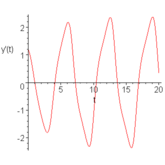
Figure 3. Plotting the approximation to the derivative of the solution to the IVP.

There appears to be a strong relationship between y(t) and y⁽¹⁾(t): this can be seen by plotting the solutions y_i, as is shown in Figure 4.

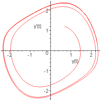
Figure 4. Plotting the vectors y_i.

These appear to be approaching a cyclic limit. If we plot the points y₁₉₃₅ through y₂₀₀₀, we note that the points form almost a perfect closed loop, as is shown in Figure 5.

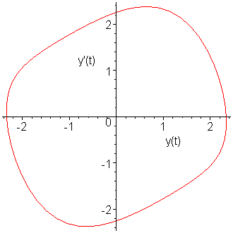
Figure 5. The limit cycle of our IVP.

Example 4

Consider a circuit with a single loop with an inductor of of 1 H, a resistor of 10 Ω and a capacitor of 0.25 F. If the system is initially at rest, and at time t = 0, a voltage force of x(t) = sin(t) for t ≥ 0 is applied. Solve for the current y(t) moving through the loop. This circuit is shown in Figure 6.

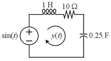
Figure 6. A linear circuit with an inductor, resistor, and a capacitor.

This system is described by the differential equation:

y⁽²⁾(t) + 10 y⁽¹⁾(t) + 4 y(t) = cos(t)
y(0) = 0
y⁽¹⁾(0) = 0

Again, we rewrite the ODE as

y⁽²⁾(t) = cos(t) − 10 y⁽¹⁾(t) − 4 y(t)

and define

with the initial conditions

The transfer function of this system is H(z) = z/(z² + 10z + 4), and therefore, the solution will approach y(t) = &re;(H(j) e^jt) = 10/109 cos(t). We will see if the numerical result is equivalent.

Seeing that cos(t) has a period of 2π, it would be appropriate to, once again, use h = 0.1. Thus, with

we find

Iterating many times, we get the approximation of the solution shown in Figure 7.

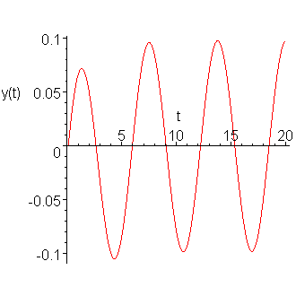
Figure 7. The solution to the forced circuit.

If we plot the approximations of the solution versus the derivative, we get the image in Figure 8.

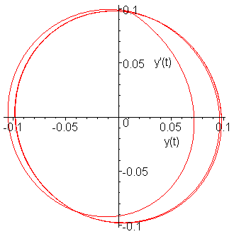
Figure 8. The solution versus the derivative.

From your circuits courses, you should expect such behaviour.

The maximum current should be 10/109 A, however, if we find the maximum approximate value of the current is 0.0980737, which is slightly greater than the expected maximum current.

Engineering

To be completed.

Error

The error analysis for higher-order differential equations is similar to that for 1st-order differential equations.

Questions

Question 1

Given the IVP shown in Example 4, find the first three iterations when then initial current -1 A. Use the value h = 0.1.

Answer: y₁ = (-1.0, 0.5)^T, y₂ = (-0.95, 0.499500)^T, y₃ = (-0.90005, 0.479500)^T.

Question 2

Given the IVP shown in Example 2, find the first three iterations when the forcing function is v(t) = e^-t for t ≥ 0. Replace the cos(t) with the derivative of the new forcing function and use h = 0.1 and assume the system is initially at rest.

Answer: y₁ = (0, -0.01)^T, y₂ = (-0.01, -0.11052)^T, y₃ = (-0.021052, -0.10652)^T.

Question 3

Consider the circuit in Figure 1.

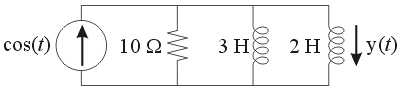
Figure 1. An RLL circuit.

From your circuits course, you can determine that the differential equation describing the current flowing across the second inductor is given by:

y⁽²⁾(t) + (10/3 + 10/2)y⁽¹⁾(t) = -10/2 sin(t)

Rewrite this as a system of 1st-order differential equations.

Question 3

Given the 3rd-order IVP

y⁽³⁾ + y⁽²⁾(t) - y⁽¹⁾(t) + y(t) + 3 = 0
y(0) = 3
y⁽¹⁾(0) = 2
y⁽²⁾(0) = 1

Approximate y(1) by using one step of Euler's method and then again, by using 2 and then 4 steps of Euler's method.

Answer: (5, 3, 2)^T; (4, 2.5, 1.5)^T and (5.25, 3.25, 1.5)^T; (3.5, 2.25, 1.25)^T, (4.0625, 2.5625, 1.375)^T, (4.703125, 2.90625, 1.40625)^T, and (5.4296875, 3.2578125, 1.35546875)^T.

Question 4

Given the 3rd-order IVP

y⁽³⁾ + ty⁽²⁾(t) - y⁽¹⁾(t) + y(t) + 3t = 0
y(0) = 3
y⁽¹⁾(0) = 2
y⁽²⁾(0) = 1

Approximate y(1) by using one step of Euler's method and then again, by using 2 and then 4 steps of Euler's method.

Answer: (5, 3, 0)^T; (4, 2.5, 0.5)^T and (5.25, 2.75, 0.375)^T; and (3.5 2.25 0.75)^T, (4.0625 2.4375 0.578125)^T, (4.671875 2.58203125 0.474609375)^T, (5.3173828125 2.70068359375 0.42565917975)^T.

Matlab

To be completed later.

Maple

Maple can solve some higher-order ODEs explicitly:

> dsolve( {
    (D@@2)(y)(t) = 4 - sin(t) + y(t) - 2*D(y)(t),
    y(0) = 1,
    D(y)(0) = 2
} );

Here, the derivative of y(t) is represented by D(y)(t) and the second derivative by (D@@2)(y)(t) (applying the derivative twice).

The second example cannot be solved by Maple, as:

> dsolve( {
    (D@@3)(y)(t) = y(t) - t*D(y)(t) + 4*(D@@2)(y)(t),
    y(0) = 1,
    D(y)(0) = 2,
    (D@@2)(y)(0) = 3
} );

returns no solution. However, you can ask for a numeric answer:

> dsolve( {
    (D@@3)(y)(t) = y(t) - t*D(y)(t) + 4*(D@@2)(y)(t),
    y(0) = 1,
    D(y)(0) = 2,
    (D@@2)(y)(0) = 3
}, 'numeric' );

                     proc(x_rkf45)  ...  end proc

From the name of the variable, you should be able to guess which method is being used to find numeric solutions to the given ODE.

For interest, Figure 1 shows a plot of the solution to the second IVP.

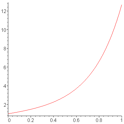
Figure 1. The solution to the 3rd-order IVP.

If we look at the initial conditions, this suggests that:

the value of the solution at 0 should be 1,
the value of the derivative at 0 should be 2, and
the concavity at 0 should be 3.

Consequently, the solution should look like the parabola with similar properties, namely

p(t) = 3/2 t² + 2 t + 1

If we plot both the solution and the parabola, we see in Figure 2 that, at 0, there is a reasonable match.

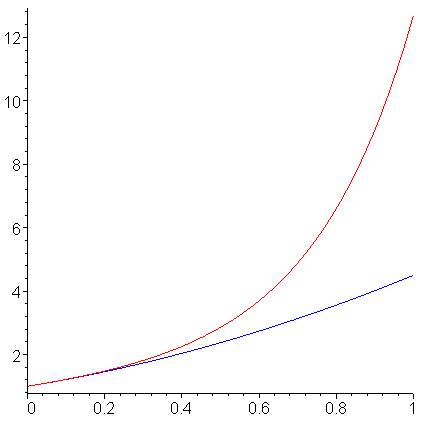
Figure 2. The solution and a fitting parabola.

Topic 14.8: Higher-Order Initial-Value Problems

Background

References

Theory

Example

HOWTO

Problem

Assumptions

Tools

Process

Examples

Example 1

Example 2

Example 3

Example 4

Engineering

Error

Questions

Question 1

Question 2

Question 3

Question 3

Question 4

Matlab

Maple