Topic 14.8: Higher-Order Initial-Value Problems (Maple)

Introduction Notes Theory HOWTO Examples Engineering Error Questions Matlab Maple

Maple can solve some higher-order ODEs explicitly:

> dsolve( {
    (D@@2)(y)(t) = 4 - sin(t) + y(t) - 2*D(y)(t),
    y(0) = 1,
    D(y)(0) = 2
} );

Here, the derivative of y(t) is represented by D(y)(t) and the second derivative by (D@@2)(y)(t) (applying the derivative twice).

The second example cannot be solved by Maple, as:

> dsolve( {
    (D@@3)(y)(t) = y(t) - t*D(y)(t) + 4*(D@@2)(y)(t),
    y(0) = 1,
    D(y)(0) = 2,
    (D@@2)(y)(0) = 3
} );

returns no solution. However, you can ask for a numeric answer:

> dsolve( {
    (D@@3)(y)(t) = y(t) - t*D(y)(t) + 4*(D@@2)(y)(t),
    y(0) = 1,
    D(y)(0) = 2,
    (D@@2)(y)(0) = 3
}, 'numeric' );

                     proc(x_rkf45)  ...  end proc

From the name of the variable, you should be able to guess which method is being used to find numeric solutions to the given ODE.

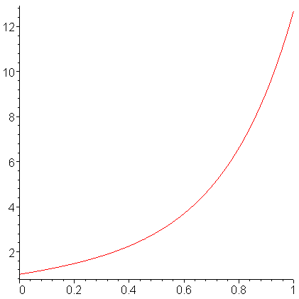
For interest, Figure 1 shows a plot of the solution to the second IVP.

Figure 1. The solution to the 3rd-order IVP.

If we look at the initial conditions, this suggests that:

the value of the solution at 0 should be 1,
the value of the derivative at 0 should be 2, and
the concavity at 0 should be 3.

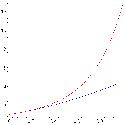
Consequently, the solution should look like the parabola with similar properties, namely

p(t) = 3/2 t² + 2 t + 1

If we plot both the solution and the parabola, we see in Figure 2 that, at 0, there is a reasonable match.

Figure 2. The solution and a fitting parabola.