

Example 1
Almost all students have seen the butterfly effect, shown here on Wikipedia.
This is the result of a system of three non-linear differential equations collectively known as the Lorenz equations:
where
These variables represent certain properties of the earth's atmosphere. If we start with an initial condition of the atmosphere, then the differential equation dictates how the properties change over time.
For demonstration purposes, we will use σ = 10, ρ = 28, and β = 2.7
If we start with the initial point u0 = (1, 1, 1)T and use the function
together with a step size of h = 0.01, then applying Euler's method, we can calculate u1:
If we repeat this 1000 times, we can plot the result, as shown in Figure 1.

Figure 1. The first 1000 approximations for the solution to the Lorenz equations (click to enlarge).
This indicates that each of the three values varies over time, however, the first two variables do not move outside the range [-20, 20] while the third variable appears to be bounded by [0, 50].
It is more common to interpolate the points, as is shown in Figure 2.
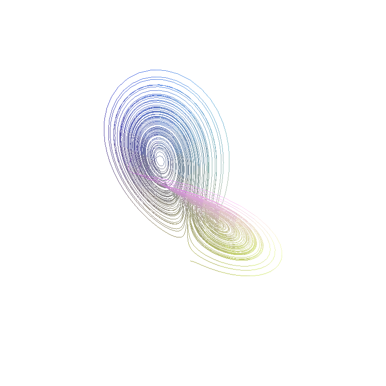
Figure 2. The first 10000 approximations for the solution to the Lorenz equations (click to enlarge).
That the solution to this differential equation follows such a peculiar path is part of the study of chaos theory.
Copyright ©2006 by Douglas Wilhelm Harder. All rights reserved.
