Introduction Notes Theory HOWTO Examples Engineering Error Questions Matlab Maple

Consider the following system of two ODEs:

x⁽¹⁾(t) = −2 x(t) − 3 y(t) + 3
y⁽¹⁾(t) = −4 x(t) − 6 y(t) − 2

where we have two initial conditions:

x(0) = −1
y(0) = 5

If we define the vector-valued function u(t) as

and then define

we may rewrite the system of ODEs as:

where f is the vector-valued function

Notice that this form is almost identical to the case with a single ODE:

y⁽¹⁾(t) = f(t, y(t))
y(t₀) = y₀

except that all of the functions u(t) and f(t, u) are now vector-valued instead of scalar-valued.

Now, whenever we did any operations in any of the methods, Euler, Huen, Runge-Kutta, or RKF45, the only operations were to:

Evaluate f(t, y) at some point (t, y) or perhaps (t + h, y + hK),
Add a scalar multiple of this onto the previous value y_k.

These are vector as well as scalar operations, and therefore, we can do the same thing with these functions.

Example

Letting h = 0.1 and using Euler's method, then

Iterating a number of times, we get the sequence u₀ through u₆ of:

If we plot the first 21 points u₀ through u₂₀, we get the points shown in Figure 1.

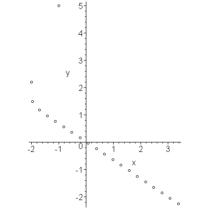
Figure 1. The first twenty approximations to the given IVP.

We can solve this IVP exactly to get that:

x(t) = 13/8 e^{−8 t} + 3 t − 21/8
y(t) = 13/4 e^{−8 t} − 2 t + 7/4

If we plot this curve for t between 0 and 2, we get the plot in Figure 2.

Figure 2. The first twenty approximations to the solution of the given IVP.

If x(t) and y(t) represent positions within a plane, then the solution u(t) = (x(t), y(t))^T represents the movement of the particle in the plane as time passes. To emphasize this, Figure 3 is an animation showing the path followed by the particle.

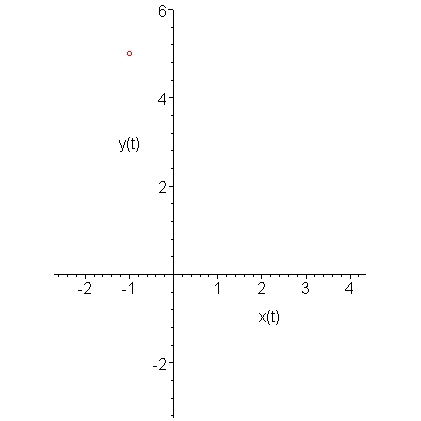
Figure 3. An animation of the solution to the IVP.

For this, we used Euler's method, however, it would not be any different to use the 4th-order Runge-Kutta method (or even RKF45). If we use a step size of h = 0, the calculation of u₁ would include:

Calculating the weighted average, we get:

Thus, the next point is

This first approximation is shown in Figure 4.

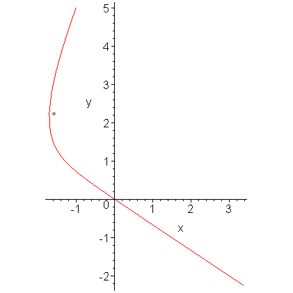
Figure 4. The first approximation using 4th-order Runge-Kutta.

If we plot the first 10 approximations, we get the points in Figure 5.

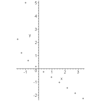
Figure 5. The first ten approximations using 4th-order Runge-Kutta.

Figure 6 compares the approximations with the actual solution. The approximations are in black while the actual values are in red. The initial significant difference between the approximations and the actual solutions and the closeness of subsequent approximations would suggest that this IVP is well suited for RKF45.

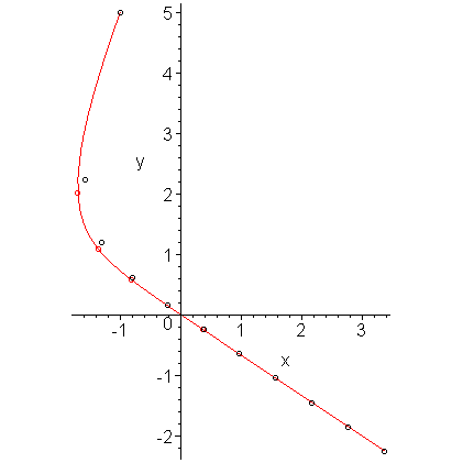
Figure 6. The approximations plotted with the actual solution.

Topic 14.7: Systems of Initial-Value Problems (Theory)

Example