Introduction Notes Theory HOWTO Examples Engineering Error Questions Matlab Maple

If the IVP is linear, that is, the function f may be written as

f(t, u) = Mu + b

for a matrix M and vector b, then we can very easily use Matlab to solve such systems.

For example, given the IVP

x⁽¹⁾(t) = -0.5 x(t) + 1.9 y(t) + 0.4
y⁽¹⁾(t) = -2.6 x(t) − 0.7 y(t) + 0.8
x(0) = 1
y(0) = 1

then we may assign M and b:

>> M = [-0.5 1.9; -2.6 0.7];
>> b = [0.4 0.8]';

We will store the iterations in the 2 × N matrix and assign the initial values to be the first column:

>> N = 10000;
>> x = zeros( 2, N );
>> x(:, 1) = [1 1]';

Next, we iterate Euler's method by assigning to the next column:

>> h = 0.01;
>> for i=2:N
     x(:, i) = x(:, i - 1) + h*(M*x(:, i - 1) + b);
end;

To plot this data, we pass plot the first row (the x values) and the second row (the y values):

>> plot( x(1, :), x(2, :) )

The result of the first 10000 iterations is shown in Figure 1.

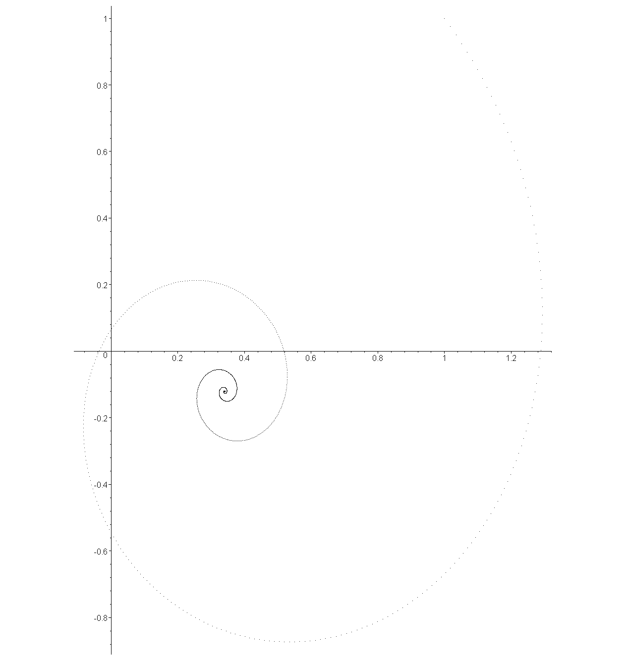
Figure 1. The first 10000 approximations of the solution to the system of IVPs (click to enlarge).

You may note that the solution appears to converge to a point. That point is the value of u such that Mu + b = 0, or Mu = −b. Thus, to find this point, we solve:

>> M \ (-b)
ans =

   0.340264650283554
  -0.120982986767486

Heun's Method

To implement Heun's method, we need only one change:

>> for i=2:N
     K0 = M*x(:, i - 1) + b;
     K1 = M*(x(:, i - 1) + h*K0) + b;
     x(:, i) = x(:, i - 1) + h*(K0 + K1)/2;
end;

4th-order Runge Kutta Method

To implement the 4th-order Runge Kutta method, we need only one change:

>> for i=2:N
     K0 = M*x(:, i - 1) + b;
     K1 = M*(x(:, i - 1) + h/2*K0) + b;
     K2 = M*(x(:, i - 1) + h/2*K1) + b;
     K3 = M*(x(:, i - 1) + h*K2) + b;
     x(:, i) = x(:, i - 1) + h*(K0 + 2*K1 + 2*K2 + K3)/6;
end;

Topic 14.7: Systems of Initial-Value Problems (Matlab)

Heun's Method

4th-order Runge Kutta Method