Topic 14.7: Systems of Initial-Value Problems (Maple)

Introduction Notes Theory HOWTO Examples Engineering Error Questions Matlab Maple

Maple works with an IVP consisting of a systems of ODEs as easily as it does with a single ODE.

dsolve( {
    D(x)(t) = -2*x(t) − y(t) + 2,
    D(y)(t) = −x(t) − 2*y(t) − 1,
    x(0) = 1,
    y(0) = 1
} );

This results in the solution

{x(t) = 5/6 e^{− 3 t}−3/2 e^−t + 5/3, y(t) = 5/6 e^{−3 t}+3/2 e^−t − 4/3}

dsolve( {
   D(x)(t) = -0.5*x(t) + 1.9*y(t) + 0.4,
   D(y)(t) = -2.6*x(t) - 0.7*y(t) + 0.8,
   x(0) = 1,
   y(0) = 1
} ):
evalf(%);

  { x(t) =  0.34026 + exp(-0.6 t) ( 0.98896 sin(2.2204 t) + 0.65973 cos(2.2204 t)),
    y(t) = -0.12098 + exp(-0.6 t) (-0.82302 sin(2.2204*t) + 1.12098 cos(2.2204 t)) }

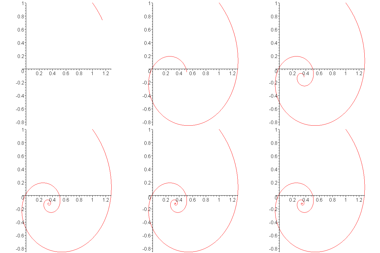
Plotting this solution for t = [0, 15], we get the result shown in Figure 1.

Figure 1. The solution to the initial value problem shown above.