The fast Fourier transform (FFT) is an algorithm which can take the discrete Fourier transform of a array of size n = 2^N in Θ(n ln(n)) time. This algorithm is generally performed in place and this implementation continues in that tradition. Two implementations are provided:

• The first implementation, FFT.basic.h, emphasizes the algorithm; consequently, to simplify the presentation, it allocates additional memory when dividing the vector into even and odd entries and explicit recursion is used, and
• The second implementation, FFT.array.h, demonstrates how the FFT algorithm can be performed with only O(1) additional memory and without recursive function calls. Reference, Maple 8, Waterloo Maple Inc., Waterloo, Ontario.

The website Fastest Fourier Transform in the West (see wikipedia for a summary) provides the fastest portable free software implementation of the FFT.

Some comments on the code:

The value π is found using double const PI = 4.0*std::atan( 1.0 ); The inverse tangent function of 1 returns π/4 and and multiplication by a power of 2 does not affect the relative error of a floating point number: in this case, multiplication by four simply adds two to the exponent.

The testing function applies the fast Fourier transform to the vector (2, 2, 0, 0, 0, 0, 0, 0)^T. It prints the vector, the fast Fourier transform of the vector, and the inverse fast Fourier transform of that result. The output is

(1,0) (1,0) (0,0) (0,0) (0,0) (0,0) (0,0) (0,0) 
(2,0) (1.70711,-0.707107) (1,-1) (0.292893,-0.707107) (0,0) (0.292893,0.707107) (1,1) (1.70711,0.707107) 
(1,0) (1,0) (0,0) (0,0) (0,0) (0,0) (0,0) (0,0) 

You will note that 1/√2 ≈ 0.707107, and 1 − 1/√2 ≈ 0.292893 .

The function printing the complex array will print 0 in place of either component being less than 10^-15. This is to make aid in the visualization of the result.

The Discrete Fourier Transform

The discrete Fourier transform maps a vector from the space domain to the complex frequency domain. To describe this, recall that a vector of n dimensions represents coordinates in space: the basis vectors are the n unit vectors (1, 0, 0, ···), (0, 1, 0, ···), etc. These are shown in Figure 1.

Figure 1. The unit basis vectors for a vector of dimension 8.

While these unit vectors are exceelent for representing the specific location of a vector, they do not suggest any periodicity. The discrete Fourier transforms is a linear transformation from a basis of unit vectors to a basis of vectors which are capture the periodic behaviour of the unit vector: if the copies of the vector were laid end-to-end, what periodicity would there be in the patterns and what are the periods thereof.

Figure 2. The basis vectors of the frequency space of dimension 8.

template <typename T> class complex<T>

This code uses the STL complex class which has a constructor which takes the real and imaginary parts as arguments. The following functions are friends of the class and for the argument z = a + jb:

Function	Returns
double abs(z)	|z| = √(a2 + b2)
double arg(z)	atan2(ℑ(z), ℜ(z)) = atan2(b, a)
complex conj(z)	z* = a − jb
double imag(z)	ℑ(z) = b
double norm(z)	|z|2 = a2 + b2
complex polar(r, θ)	rejθ
double real(z)	ℜ(z) = a
complex exp(z)	ez
complex log(z)	ln(z)
complex pow(w, z)	wz
complex sqrt(z)	√z
complex sin(z)	sin(z)
complex cos(z)	cos(z)
complex sinh(z)	sinh(z)
complex cosh(z)	cosh(z)

A complex number a + jb is printed as the ordered pair (a,b).

Determining Powers of Two

The assertion assert( n > 0 && (n & (~n + 1)) == n ); checks to ensure that the argument n is both positive and a power of two. The operation n & (~n + 1) selects the least significant one in the integer. If the least significant one is also the most significant one, then the bitwise and will return that value; otherwise, the result will not equal the original value n. This is shown in Figure 3 with both a power of two (64) and a number which is not a power of two (84).

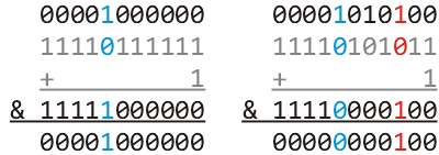
Figure 3. Selecting the least significant one (1) bit in a binary number.