A Newton polynomial which interpolates n points (x₁, y₁), ..., (x_n, y_n) is defined according to the formula shown in Figure 1.

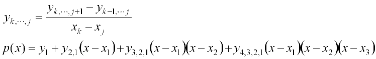
Figure 1. The definition of the Newton polynomial coefficients and the resulting polynomial passing through four points.

The coefficients of a Newton polynomial are calculated using a table of divided differences. This is an application of dynamic programming—by simply using the the definition of the coefficients of the Newton polynomial, this would produce a formula which may be described by T(n) = 2T(n − 1) + Θ(1) which implies that the function has T(n) = Θ(2ⁿ) calculations and therefore an exponential run time; however, many of these calculations are repeated. These repeated subproblems are the hallmark of an algorithm suitable for a dynamic program. Figure 2 demonstrates the table of divided differences with the Newton polynomial coefficients circled in red.

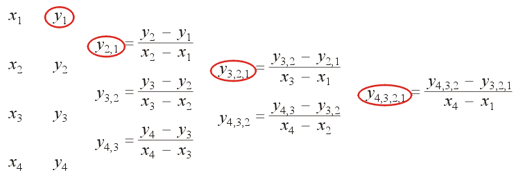
Figure 2. The table of divided differences for finding the Newton polynomial passing through four points.

Run-Time

Using a divided-difference table, the run-time for calculating the coefficients of the Newton polynomial is reduced to Θ(n²).

Memory

The divided-difference table has Θ(n²) entries; however, with the exception of the first entry which is one of the coefficients of the Newton polynomial, once the balance of the first column has been used to calculate the second, those values are no longer required. Consequently, the coefficients of the Newton polynomial using the divided-difference table may be calculated with Θ(n) memory. This is demonstrated in Figure 3.

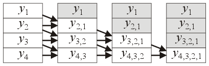
Figure 3. Calculating the Newton polynomial coefficients in a single array of size n.

Extending Newton Polynomials

The exception to this observation is when one is using Newton polynomials with time series: for example, given the points (x₁, y₁), ..., (x_n, y_n), and having calculated the Newton polynomial for these n points, given the next point (x_n + 1, y_n + 1), we may wish to calculate the Newton polynomial of the same degree but passing through the points (x₂, y₂), ... (x_n, y_n), (x_n + 1, y_n + 1). This may be done by reusing a significant portion of the previously calculated divided difference table; it requires the calculation of only one more diagonal as is shown in Figure 4 which adds a fifth point onto the table of divided differences.

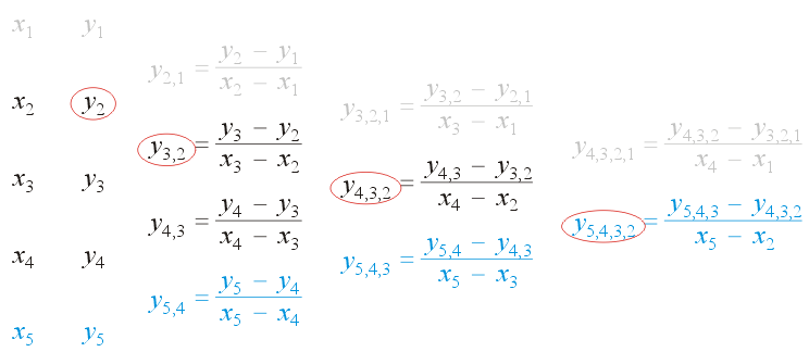
Figure 4. Adding one more point onto the table of divided differences.

One should be warned against calculating a polynomial of degree four in this case: the higher the degree of the polynomial, the more likely the error is to be magnified. The reader is asked to read any suitable reference on polynomial wiggle and Runge's phenomenon.

By storing the divided-difference table, it is possible to calculate the new Newton polynomial in Θ(n) time but it requires that the entire table be kept in memory: Θ(n²). The updated table of divided differences is shown in Figure 5.

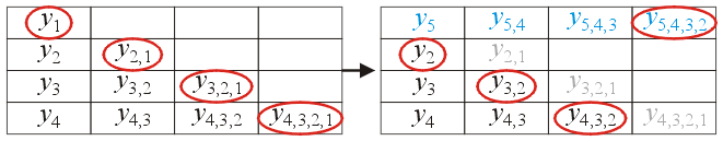
Figure 5. Updating the table of divided differences to calculate the Newton polynomial interpolating through the second through fifth points.

Horner's Rule

As a side note, many text books teach Newton polynomials without teaching the only efficient means of evaluating these polynomials: Horner's rule. This allows numerically stable evaluation with Θ(1) memory and Θ(n) time.

Dynamic Evaluation

One feature of Newton polynomials not often explained nor demonstrated is the construction of the Newton polynomial from the divided-difference table. The divided-difference table gives 2^N − 1 different paths of construction, all of which define an interpolating polynomial of the same N points. To minimize the error, one must evaluate that path which starts from the tip of the triangle and moves in the direction away from the x-value furthest from the point being evaluated. This avoids a multiplication by the largest term of the form (x − x_j). This ensures that successive terms in the Newton polynoimal decay quickly leaving the y_k closest to the point of evaluation plus the smallest possible correction with a linear term.

Specifically, if the x values are ordered, the optimal interpolating Newton polynomial to evaluate a point in the neighbourhood of the first point is

y₁ + y₂₁(x − x₁) + y₃₂₁(x − x₁)(x − x₂) + y₄₃₂₁(x − x₁)(x − x₂)(x − x₃)

Such an evaluation may be found using evaluate( x, BACKWARD ), as we are traversing the upper edge of the divided-difference table back towards the least-recently added point.

The optimal interpolating Newton polynomial to evaluate a point in the neighbourhood of the last point is

y₄ + y₄₃(x − x₄) + y₄₃₂(x − x₄)(x − x₃) + y₄₃₂₁(x − x₄)(x − x₃)(x − x₂)

Such an evaluation may be found using evaluate( x, FORWARD ), as we are traversing the lower edge of the divided-difference table towards the most-recently added point.

Suppose, however, that the four x-values are ordered and equally spaced and the point of evaluation is close to, but less than the 3rd point. In this case, the optimal interpolating Newton polynomial would be:

y₃ + y₃₂(x − x₃) + y₄₃₂(x − x₃)(x − x₂) + y₄₃₂₁(x − x₃)(x − x₂)(x − x₄)

This selection may be done with Θ(1) additional work (a comparison of two float differences) and therefore does not asymptotically affect the run time. From experiments, it increases the run time by less than a factor of 2 (approximately 80%). See the implementation for details.

To demonstrate this, Figures 6, 7, and 8 show the error of evaluating the Newton polynomial at 4097 points on [2, 6] using the forward, backward, and closest evaluating methods for the polynomial interpolating (2, sin(2)), (3, sin(3)), (4, sin(4)), (5, sin(5)), and (6, sin(6)). In the forward case, the evaluation of the points near x = 2 has the least numerical error; while in the backward case, the evaluation near x = 6 has the least error.

Figure 6. The absolute error of evaluating the Newton polynomial in the forward direction.

Figure 7. The absolute error of evaluating the Newton polynomial in the backward direction.

Figure 8. The absolute error of evaluating the optimal Newton polynomial for each point.

Note that this is not the error between the polynomial and the function being interpolated (in this case, sin(x)), but rather the error between the evaluated double-precision floating-point number and the actual value of the interpolating polynomial which explicitly interpolates the given points. Note also that these display the absolute error: for evaluating values of sin(x) where |sin(x)| is small, the absolute error is also small.

Optimization on Path Choice

If the points are ordered spaced, there are only 2(N − 1) paths which would be used to construct the Newton polynomial. For example, Figure 9 shows the six possible Newton polynomials which optimally evaluate values of x on various subintervals.

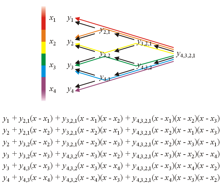
Figure 9. The six possible optimal Newton polynomials for evaluating various values of x.

If the points are ordered and equally spaced, the choice of path may be determined by the formula Δ = (x_n − x₁)/(n − 1) and min( max( 0, floor( (x - x₁)/Δ + 1 ) ), 2n - 1 ).

If the points are unordered, such a restriction to the number of paths would not be possible.

Figure 10 shows the eight possible paths of evaluation for the interpolating Newton polynomials on five ordered spaced points.

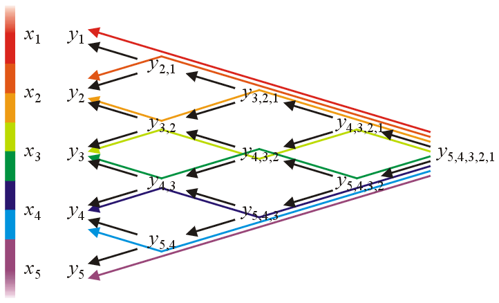
Figure 10. The eight possible optimal Newton polynomials for evaluating various values of x for interpolating five points.

Comparing Optimal Newton Polynomial Evaluation and Simple Polynomial Evaluation

The expanded polynomial interpolating the five points is

.

Figure 11 shows the errors when evaluating this expanded polynomial at points on the interval in magenta and the optimal Newton polynomial evaluation. In almost all cases, the optimal Newton polynomial evaluation produces the closest floating-point number to the actual value of the polynomial evaluated at that point. Using standard evaluation of the expanded polynomial, the error can be 200% higher, and this is is under almost ideal conditions.

Figure 11. The errors when evaluating the optimal Newton polynomial (black) and the evaluation of the expanded polynomial for the five points .

Note that these are almost ideal conditions for evaluating expanded polynomials. The error for more standard cases is much higher.

Newton Polynomial
class Newton_polynomial<N, Type = double>

Constructors

Newton_polynomial<N, Type>()

The constructor initializes the state to the default zero polynomial. It will store the coefficients of the Newton polynomial which passes through the last N points. It requires Θ(n²) memory.

Accessors

Type evaluate( Type const &x, direction dir = OPTIMAL ) const

Evaluate the Newton polynomial at the point x using Horner's rule. The second argument defines the method of construction of the Newton polynomial: for ordered values of x and an evaluation closest to the most recently added point, use FORWARD, for an evaluation closest to the least recently added point, use BACKWARD, and to use the most numerically stable dynamic construction of the Newton polynomial for any situation other than those two already mentioned, use OPTIMAL. (O(N) time and Θ(1) memory)

Type x( int k ) const

Returns the entry x_k where the order of the x-values are x₀, x₁, ... x_N − 1 with the first being the least recently added and the last being the most recently added.

Type y( int j, int k ) const

Returns the entry y_{j, ..., k} where y_{k, k} is the y value corresponding to the x value x_k and other values may be calculated as shown above.

Mutators

void insert( Type const &x, Type const &y )

Insert a new point (x, y) and calculate the coefficients of the Newton polynomial passing through the last N points. The evaluation of Newton polynomials is most numerically stable when the point x is closest to the least recently inserted x-value. (O(N) time and Θ(1) memory)

void clear()

Reset the polynomial to the zero polynomial passing through no points. (Θ(1))